Assimilation Algorithms EDA and Hybrid Data Assimilation Massimo

Assimilation Algorithms: EDA and Hybrid Data Assimilation Massimo Bonavita ECMWF Massimo. Bonavita@ecmwf. int Acknowledgements to Lars Isaksen, Elias Holm, Mike Fisher 1

Outline • A variational implementation of the En. KF: the EDA • Hybrid Data Assimilation: Motivation • Hybrid Data Assimilation systems in global NWP 2

The Ensemble of Data Assimilations (EDA) • In the previous lecture on Ensemble Kalman Filters we have seen that En. KF are commonly used in hybrid DA systems for estimating and cycling error covariance information used by the variational analysis and initialise ensemble prediction systems • Ensemble sizes of O(100 -200) are commonly used. To save on computational expense the En. KF ensemble is run at a reduced spatial resolution with respect to the deterministic variational analysis cycle

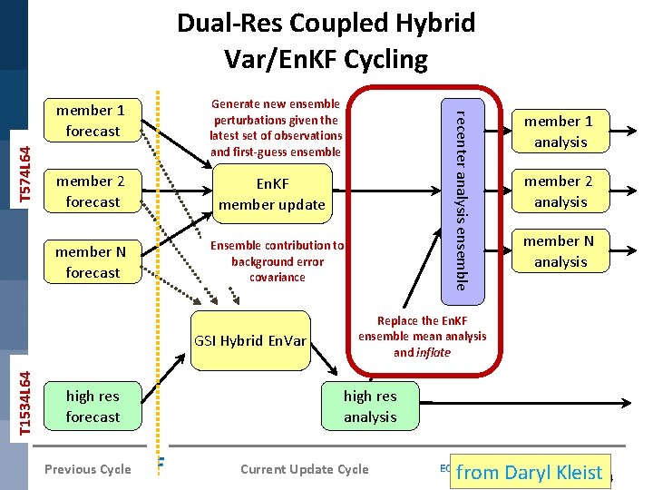
member 1 forecast Generate new ensemble perturbations given the latest set of observations and first-guess ensemble member 2 forecast En. KF member update member N forecast Ensemble contribution to background error covariance T 1534 L 64 GSI Hybrid En. Var high res forecast Previous Cycle recenter analysis ensemble T 574 L 64 Dual-Res Coupled Hybrid Var/En. KF Cycling member 1 analysis member 2 analysis member N analysis Replace the En. KF ensemble mean analysis and inflate high res analysis Current Update Cycle from Daryl Kleist 4

The Ensemble of Data Assimilations (EDA) • In the previous lecture on Ensemble Kalman Filters we have seen that En. KF are commonly used in hybrid DA systems for estimating and cycling error covariance information used by the variational analysis and initialise ensemble prediction systems • Ensemble sizes of O(100 -200) are commonly used. To save on computational expense the En. KF ensemble is run at a reduced spatial resolution wrto the deterministic variational analysis cycle • Can we replicate the error cycling job done by the En. KF using only 4 D-Var?

The Ensemble of Data Assimilations (EDA) • Can we replicate the error cycling job done by the En. KF using only 4 D-Var? • Yes, by applying the same error simulation concepts used for the stochastic (perturbed observations) En. KF • Ensemble of Data Assimilations (EDA; Isaksen et al. , 2007)

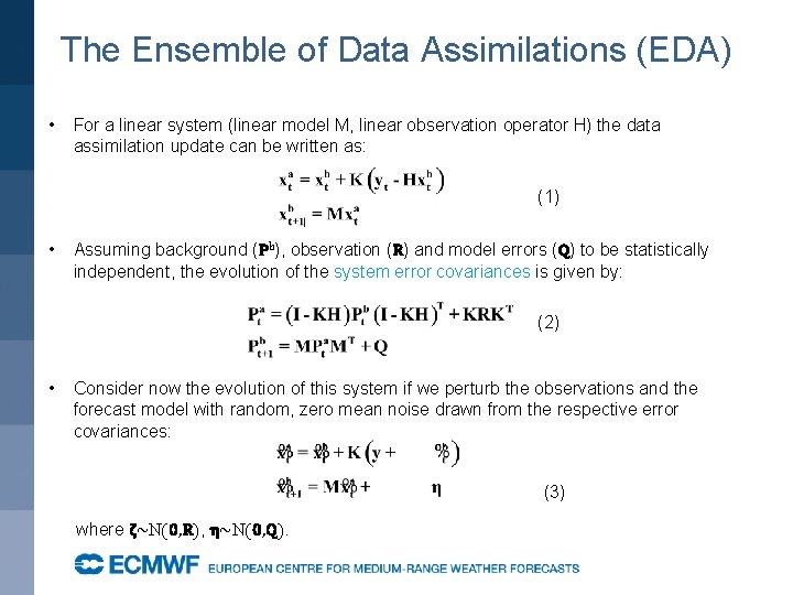
The Ensemble of Data Assimilations (EDA) • For a linear system (linear model M, linear observation operator H) the data assimilation update can be written as: (1) • Assuming background (Pb), observation (R) and model errors (Q) to be statistically independent, the evolution of the system error covariances is given by: (2) • Consider now the evolution of this system if we perturb the observations and the forecast model with random, zero mean noise drawn from the respective error covariances: (3) where ζ~N(0, R), η~N(0, Q).

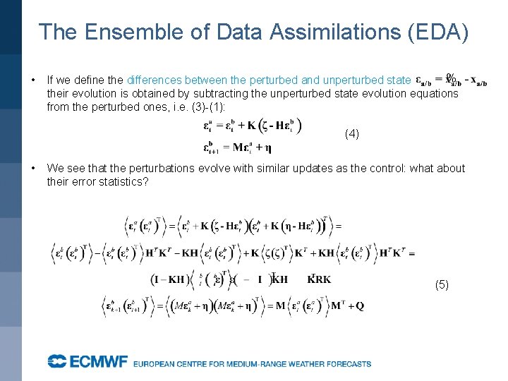
The Ensemble of Data Assimilations (EDA) • If we define the differences between the perturbed and unperturbed state their evolution is obtained by subtracting the unperturbed state evolution equations from the perturbed ones, i. e. (3)-(1): (4) • We see that the perturbations evolve with similar updates as the control: what about their error statistics? (5)

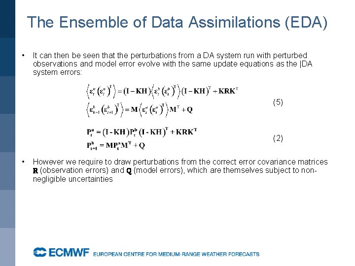
The Ensemble of Data Assimilations (EDA) • It can then be seen that the perturbations from a DA system run with perturbed observations and model error evolve with the same update equations as the |DA system errors: (5) (2) • However we require to draw perturbations from the correct error covariance matrices R (observation errors) and Q (model errors), which are themselves subject to nonnegligible uncertainties

The Ensemble of Data Assimilations (EDA) • What does all this mean in practice? 1. We can use an ensemble of perturbed data assimilation cycles to simulate the errors of our reference DA cycle; 2. The ensemble of perturbed DAs should be as similar as possible to the reference DA (i. e. , same or similar K matrix, M, H, and resolution) 3. The applied perturbations ζ , η should have the correct error covariances (R, Q); 4. There is no need to explicitly perturb the background forecast xb 5. This is a Monte Carlo method: the expectation operator used in (5) implies that results strictly hold for infinite ensemble sizes. In practice non-negligible sampling errors are to be expected

The Ensemble of Data Assimilations (EDA) • What does all this mean in practice? 1. 25 ensemble members using 4 D-Var assimilations at reduced resolution 2. TCo 639 outer loop, TL 191/TL 191 inner loops. (Reference DA: TCo 1279 outer loop, TL 255/TL 319/TL 399 inner loops). 3. Observations randomly perturbed according to their estimated error covariances (R) 4. SST perturbed with climatological error structures 5. Model error (Q) represented by stochastic perturbations during the background forecast integration (SPPT, Leutbecher, 2009)

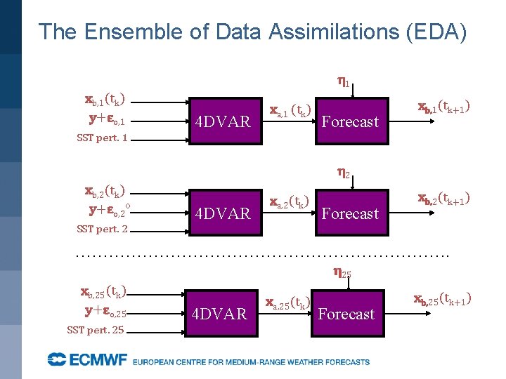
The Ensemble of Data Assimilations (EDA) η 1 xb, 1(tk) y+εo, 1 4 DVAR xa, 1 (tk) Forecast xb, 1(tk+1) SST pert. 1 η 2 xb, 2(tk) y+εo, 2 o 4 DVAR xa, 2(tk) Forecast xb, 2(tk+1) SST pert. 2 ……………………………. η 25 xb, 25(tk) y+εo, 25 SST pert. 25 4 DVAR xa, 25(tk) Forecast xb, 25(tk+1)

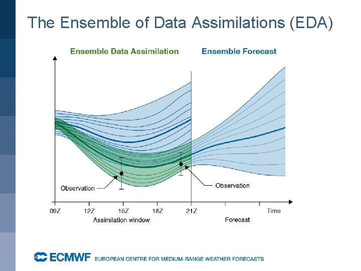
The Ensemble of Data Assimilations (EDA) • The EDA simulates the error evolution of the 4 DVar analysis cycle. As such it has two main applications: 1. Provide an ensemble of initial conditions to initialize the ensemble prediction system 2. Provide a flow-dependent estimate of background error covariances for use in the 4 D-Var assimilation (both for the HRES DA system and the EDA members themselves)

The Ensemble of Data Assimilations (EDA)

The Ensemble of Data Assimilations (EDA) • The EDA is the system used at ECMWF to simulate the error evolution of the 4 DVar analysis cycle. • It is conceptually similar and it is based on the same assumptions of a Perturbed Observations (Stochastic) En. KF. • There advantages to using an ensemble of 4 DVar to simulate the error of a reference high resolution 4 DVar: 1. The two systems are more similar to one another in terms of Kalman Gain than an En. KF and a 4 DVar; error estimates should thus be more accurate 2. There are technical and maintenance synergies • There also some disadvantages. In particular running an ensemble of 4 DVar is considerably more expensive than running an En. KF. Current efforts are aimed at reducing the computational costs of the EDA in order to make a larger ensemble computationally affordable

Hybrid Data Assimilation •

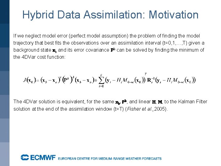
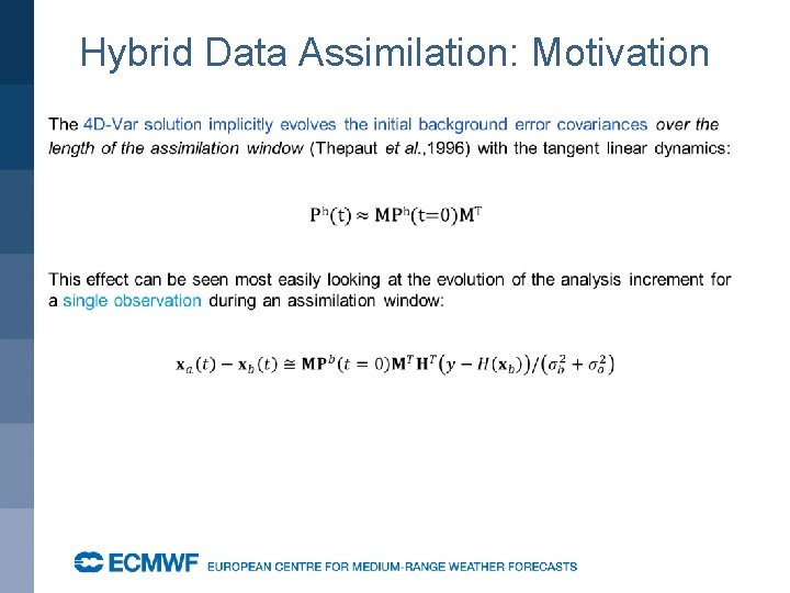
Hybrid Data Assimilation: Motivation If we neglect model error (perfect model assumption) the problem of finding the model trajectory that best fits the observations over an assimilation interval (t=0, 1, …, T) given a background state xb and its error covariance Pb can be solved by finding the minimum of the 4 DVar cost function: The 4 DVar solution is equivalent, for the same xb, Pb, and linear H, M, to the Kalman Filter solution at the end of the assimilation window (t=T) (Fisher et al. , 2005).

Hybrid Data Assimilation: Motivation

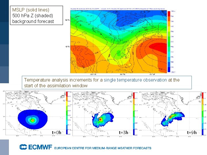
MSLP (solid lines) 500 h. Pa Z (shaded) background forecast Temperature analysis increments for a single temperature observation at the start of the assimilation window t=0 h t=3 h t=9 h

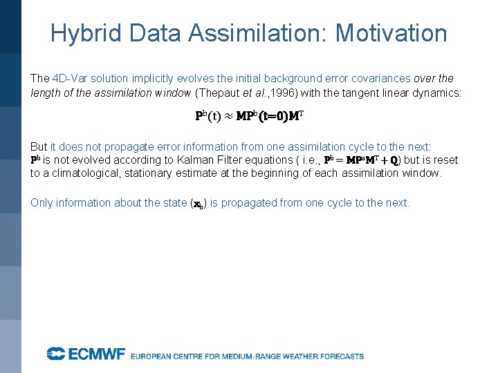
Hybrid Data Assimilation: Motivation The 4 D-Var solution implicitly evolves the initial background error covariances over the length of the assimilation window (Thepaut et al. , 1996) with the tangent linear dynamics: Pb(t) ≈ MPb(t=0)MT But it does not propagate error information from one assimilation cycle to the next: Pb is not evolved according to Kalman Filter equations ( i. e. , Pb = MPa. MT + Q) but is reset to a climatological, stationary estimate at the beginning of each assimilation window. Only information about the state (xb) is propagated from one cycle to the next.

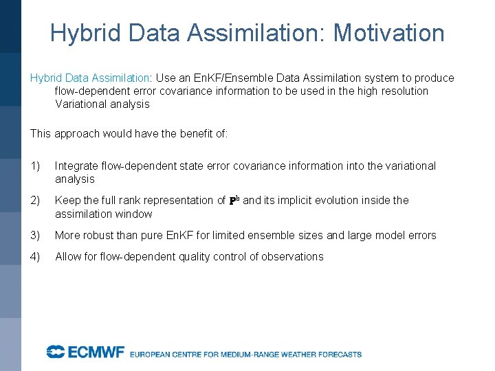
Hybrid Data Assimilation: Motivation Hybrid Data Assimilation: Use an En. KF/Ensemble Data Assimilation system to produce flow-dependent error covariance information to be used in the high resolution Variational analysis This approach would have the benefit of: 1) Integrate flow-dependent state error covariance information into the variational analysis 2) Keep the full rank representation of Pb and its implicit evolution inside the assimilation window 3) More robust than pure En. KF for limited ensemble sizes and large model errors 4) Allow for flow-dependent quality control of observations

Hybrid Data Assimilation: Applications The next question to address is: how do we integrate the flow-dependent error covariance information from the En. KF/EDA systems into the variational analysis? 1. Extended control variable method (Met Office) 2. 4 D-Ensemble-Var (NCEP, CMC, DWD) 3. Hybrid EDA 4 D-Var (ECMWF, Météo France)

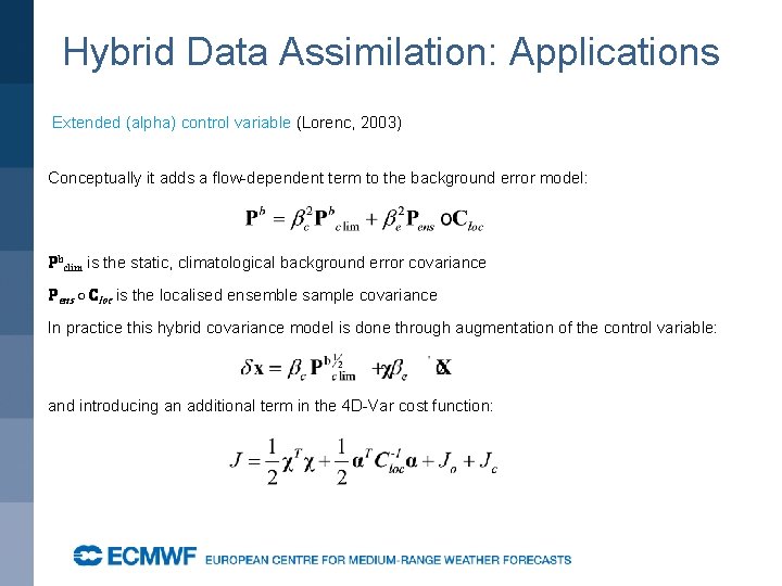
Hybrid Data Assimilation: Applications Extended (alpha) control variable (Lorenc, 2003) Conceptually it adds a flow-dependent term to the background error model: Pbclim is the static, climatological background error covariance Pens ○ Cloc is the localised ensemble sample covariance In practice this hybrid covariance model is done through augmentation of the control variable: and introducing an additional term in the 4 D-Var cost function:

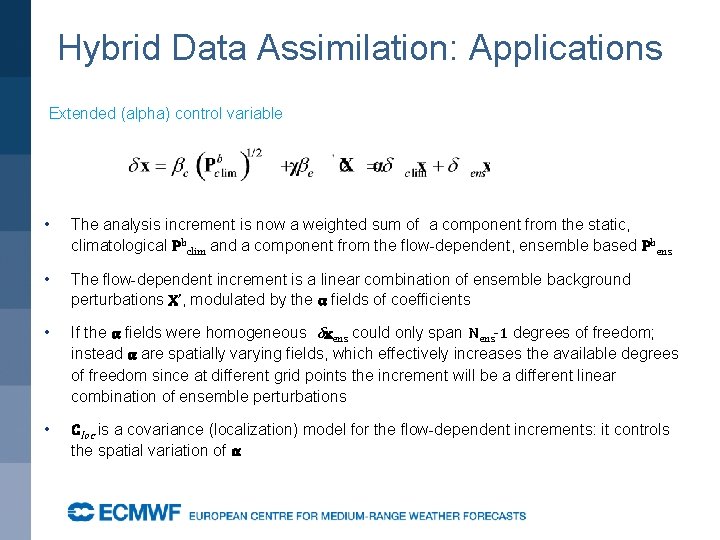
Hybrid Data Assimilation: Applications Extended (alpha) control variable • The analysis increment is now a weighted sum of a component from the static, climatological Pbclim and a component from the flow-dependent, ensemble based Pbens • The flow-dependent increment is a linear combination of ensemble background perturbations X’, modulated by the α fields of coefficients • If the α fields were homogeneous δxens could only span Nens-1 degrees of freedom; instead α are spatially varying fields, which effectively increases the available degrees of freedom since at different grid points the increment will be a different linear combination of ensemble perturbations • Cloc is a covariance (localization) model for the flow-dependent increments: it controls the spatial variation of α

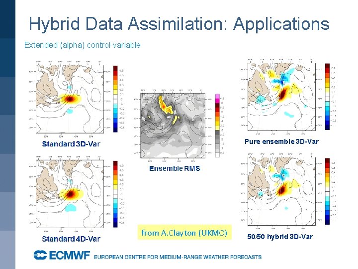
Hybrid Data Assimilation: Applications Extended (alpha) control variable Pure ensemble 3 D-Var from A. Clayton (UKMO) 50/50 hybrid 3 D-Var

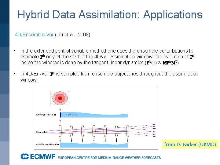
Hybrid Data Assimilation: Applications 4 D-Ensemble-Var (Liu et al. , 2008) • In the extended control variable method one uses the ensemble perturbations to estimate Pb only at the start of the 4 DVar assimilation window: the evolution of Pb inside the window is done by the tangent linear dynamics (Pb(t) ≈ MPb. MT) • In 4 D-En-Var Pb is sampled from ensemble trajectories throughout the assimilation window: from D. Barker (UKMO)

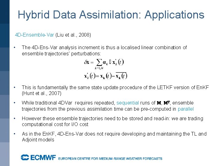
Hybrid Data Assimilation: Applications 4 D-Ensemble-Var (Liu et al. , 2008) • The 4 D-Ens-Var analysis increment is thus a localised linear combination of ensemble trajectories’ perturbations: • This is fundamentally the same state update procedure of the LETKF version of En. KF (Hunt et al. , 2007) • While traditional 4 DVar requires repeated, sequential runs of M, MT, ensemble trajectories from the previous assimilation time can be pre-computed in parallel • However these ensemble trajectories need to be stored and read-in: we are trading computational cost for I/O cost • As in the En. KF, 4 D-Ens-Var does not require developing and maintaining the TL and Adjoint models

Hybrid Data Assimilation: Applications Hybrid EDA 4 D-Var (Isaksen et al. , 2007; Bonavita et al. , 2012, 2015) • In Hybrid 4 D-Var we use the perturbations from the EDA background forecasts to update the background error covariance model used in 4 D-Var • The ensemble perturbations are not used directly to construct the analysis increments, but to update the Pb used in 4 D-Var

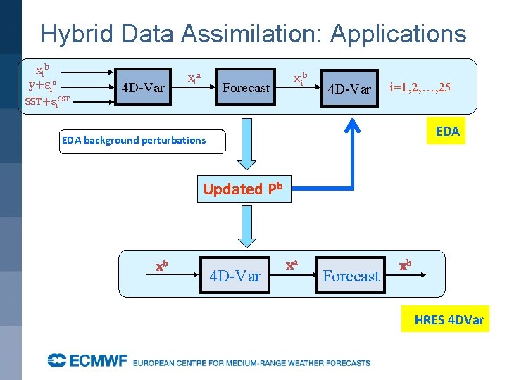
Hybrid Data Assimilation: Applications xib y+εio 4 D-Var xia Forecast xib SST+εi. SST 4 D-Var i=1, 2, …, 25 EDA background perturbations Updated Pb xb 4 D-Var xa Forecast xb HRES 4 DVar

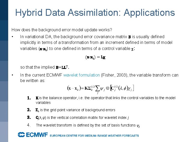
Hybrid Data Assimilation: Applications How does the background error model update works? • In variational DA, the background error covariance matrix B is usually defined implicitly in terms of a transformation from an increment defined in terms of model variables (x-xb) to one defined in terms of a control variable χ: (x-xb) = Lχ so that the implied B=LLT. • In the current ECMWF wavelet formulation (Fisher, 2003), the variable transform can be written as: 1. K is the balance operator, i. e. the operator that links the control variables to the model variables 2. Σb is the grid point variance of background errors 3. Cj(λ, φ) is the vertical correlation matrix for wavelet index j 4. The wavelet transform is defined by the set of basis functions ψj

Hybrid Data Assimilation: Applications How does the background error model update works? • In standard 4 D-Var the background error variances (Σb) and the background error correlations (Cj(λ, φ)) are computed offline from a climatology of EDA background perturbations. • In Hybrid EDA 4 D-Var these quantities are updated using the latest set of EDA background perturbations • In this way the B model is continuously updated and is able to represent the “errors of the day”

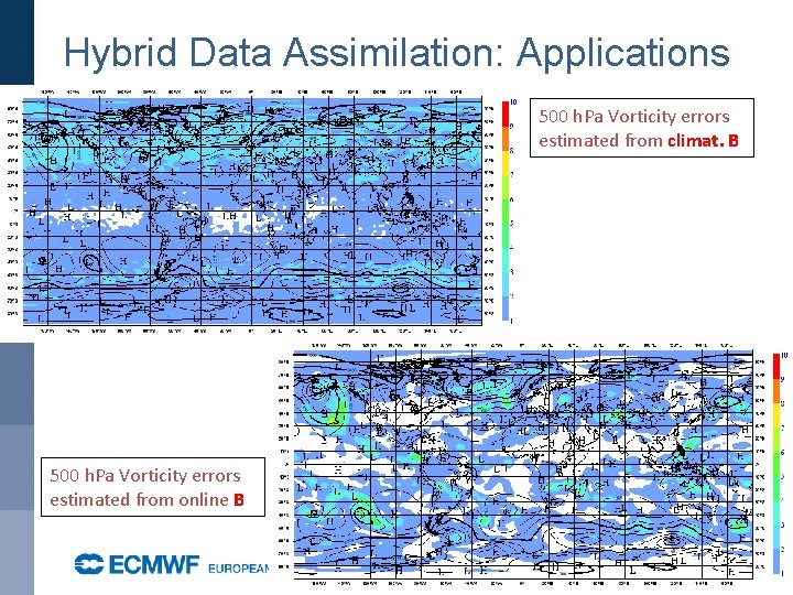
Hybrid Data Assimilation: Applications How does the background error model update works? 500 h. Pa Vorticity errors estimated from online B 500 h. Pa Vorticity errors estimated from climat. B

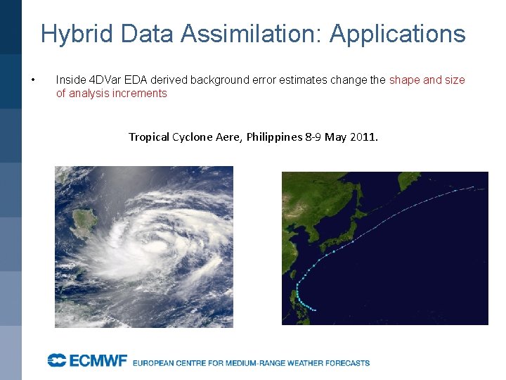
Hybrid Data Assimilation: Applications • Inside 4 DVar EDA derived background error estimates change the shape and size of analysis increments Tropical Cyclone Aere, Philippines 8 -9 May 2011.

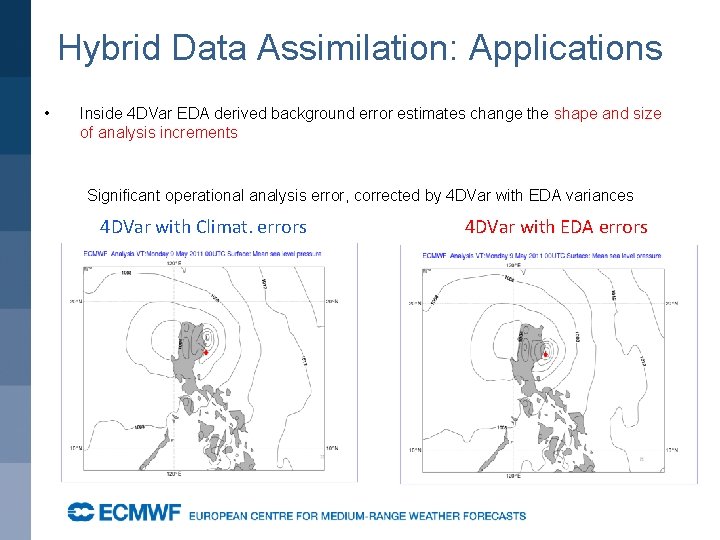
Hybrid Data Assimilation: Applications • Inside 4 DVar EDA derived background error estimates change the shape and size of analysis increments Significant operational analysis error, corrected by 4 DVar with EDA variances 4 DVar with Climat. errors 4 DVar with EDA errors

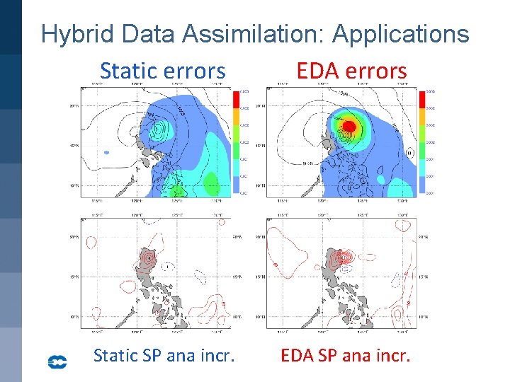
Hybrid Data Assimilation: Applications Static errors EDA errors Static SP ana incr. EDA SP ana incr.

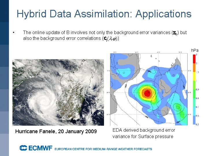
Hybrid Data Assimilation: Applications • The online update of B involves not only the background error variances (Σb) but also the background error correlations (Cj(λ, φ)) h. Pa Hurricane Fanele, 20 January 2009 EDA derived background error variance for Surface pressure

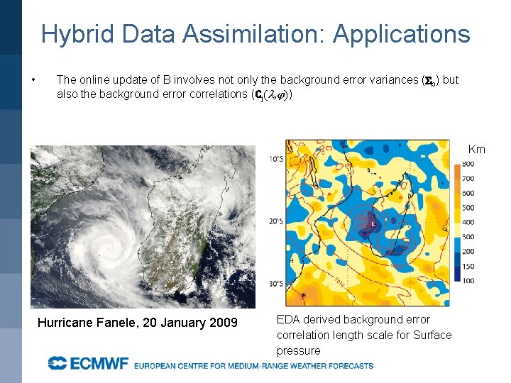
Hybrid Data Assimilation: Applications • The online update of B involves not only the background error variances (Σb) but also the background error correlations (Cj(λ, φ)) Km Hurricane Fanele, 20 January 2009 EDA derived background error correlation length scale for Surface pressure

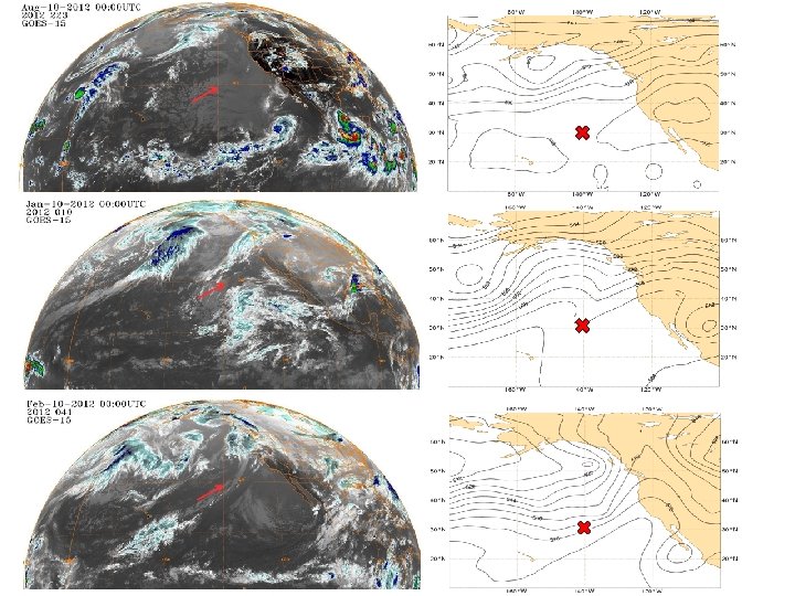
Wavelet B Computation

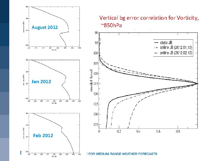
August 2012 Jan 2012 Feb 2012 Vertical bg error correlation for Vorticity, ~850 h. Pa

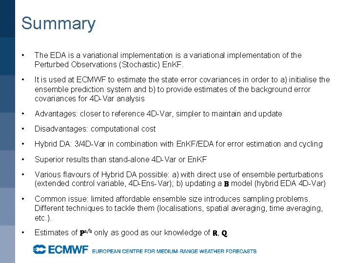
Summary • The EDA is a variational implementation of the Perturbed Observations (Stochastic) En. KF. • It is used at ECMWF to estimate the state error covariances in order to a) initialise the ensemble prediction system and b) to provide estimates of the background error covariances for 4 D-Var analysis • Advantages: closer to reference 4 D-Var, simpler to maintain and update • Disadvantages: computational cost • Hybrid DA: 3/4 D-Var in combination with En. KF/EDA for error estimation and cycling • Superior results than stand-alone 4 D-Var or En. KF • Various flavours of Hybrid DA possible: a) with direct use of ensemble perturbations (extended control variable, 4 D-Ens-Var); b) updating a B model (hybrid EDA 4 D-Var) • Common issue: limited affordable ensemble size introduces sampling problems. Different techniques to tackle them (localisations, spatial averaging, time averaging, etc. ). • Estimates of Pa/b only as good as our knowledge of R, Q.

Bibliography 1. Bonavita M. , L. Raynaud and L. Isaksen, 2010: Estimating background-error variances with the ECMWF Ensemble of Data Assimilations system: the effect of ensemble size and day-to-day variability. Q. J. R. Meteorol. Soc. , 137: 423– 434. 2. Bonavita M. , L. Isaksen and E. Holm, 2012: On the use of EDA background error variances in the ECMWF 4 D-Var. Q. J. R. Meteorol. Soc. . Early Online Release, doi: 10. 1002/qj. 1899 3. Bonavita M. , E. Holm, L. Isaksen and M. Fisher, 2015: The evolution of the ECMWF hybrid data assimilation system, Q. J. R. Meteorol. Soc. , 142: 287– 303. DOI: 10. 1002/qj. 2652. 4. Fisher, M. Leutbecher M, Kelly GA. 2005 On the equivalence between Kalman smoothing and weak-constraint four-dimensional variational data assimilation. Q. J. R. Meteorol. Soc. 131 3235– 3246. 5. Fisher, M. , 2003: Background error covariance modelling. Proceedings of the ECMWF Seminar on recent developments in data assimilation for atmosphere and ocean, ECMWF, pages 45– 63. (Available from: http: //www. ecmwf. int/publications/) 6. Isaksen, L. , M. Bonavita, R. Buizza, M. Fisher, J. Haseler, M. Leutbecher and Laure Raynaud, 2010: Ensemble of data assimilations at ECMWF Technical Memorandum No. 636. (Available from: http: //www. ecmwf. int/publications/)

Bibliography 7. Hunt, B. R. , Kostelich, E. J. and Szunyogh, I. , 2007. Efficient data assimilation for spatiotemporal chaos: a local ensemble transform Kalman filter. Physica D, 230, 112– 126. 8. Liu C, Xiao Q, Wang B. 2008. An ensemble-based four-dimensional variational data assimilation scheme. part i: Technical formulation and preliminary test. Mon. Weather Rev. 136: 3363– 3373. 9. Lorenc, A. C. , 2003: The potential of the ensemble Kalman filter for NWP—A comparison with 4 D-VAR. Q. J. R. Meteorol. Soc. , 129: 3183– 3203. 10. Ott E, Hunt BR, Szunyogh I, Zimin AV, Kostelich EJ, Corazza M, Kalnay E, Patil DJ. 2004. A local ensemble Kalman filter for atmospheric data assimilation. Tellus 56 A: 415– 428. 11. Raynaud, L. Berre, and G. Desroziers, 2008: Spatial averaging of ensemble-based background-error variances. Q. J. R. Meteorol. Soc. , 134, 1003– 1014. 12. Thepaut, J. -N. , Courtier, P. , Belaud, G. and Lemaıtre, G. , 1996: Dynamical structure functions in a four-dimensional variational assimilation: A case study. Q. J. R. Meteorol. Soc. , 122, 535– 561