Forecast 2 Linear trend Forecast error Seasonal demand

Forecast 2 Linear trend Forecast error Seasonal demand

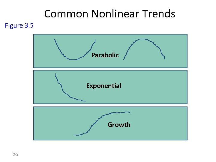
Common Nonlinear Trends Figure 3. 5 Parabolic Exponential Growth 3 -2

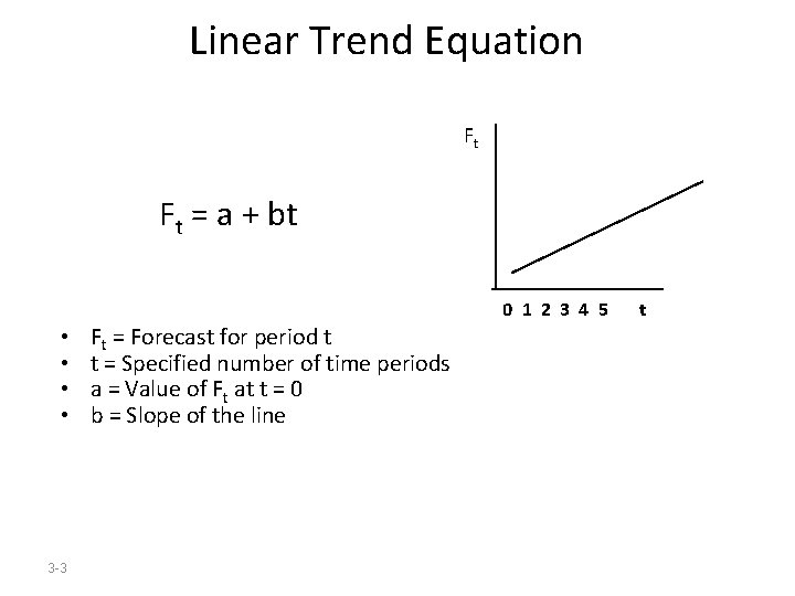
Linear Trend Equation Ft Ft = a + bt 0 1 2 3 4 5 • • 3 -3 Ft = Forecast for period t t = Specified number of time periods a = Value of Ft at t = 0 b = Slope of the line t

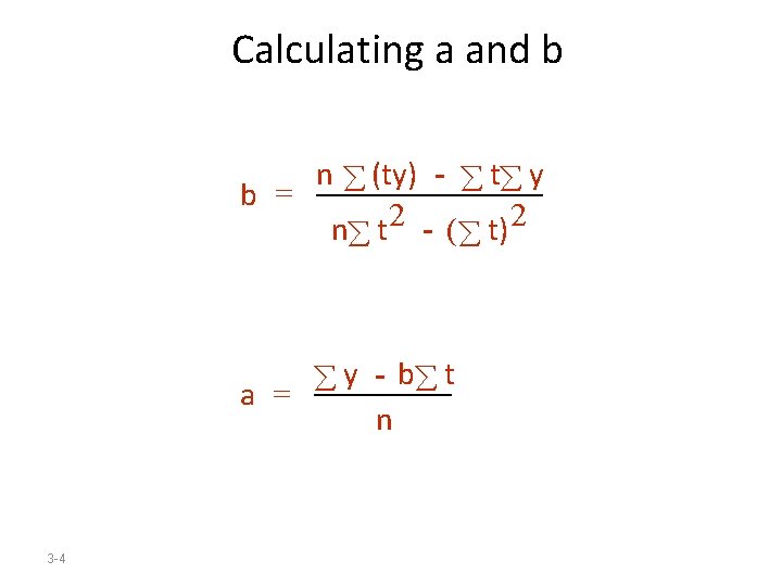
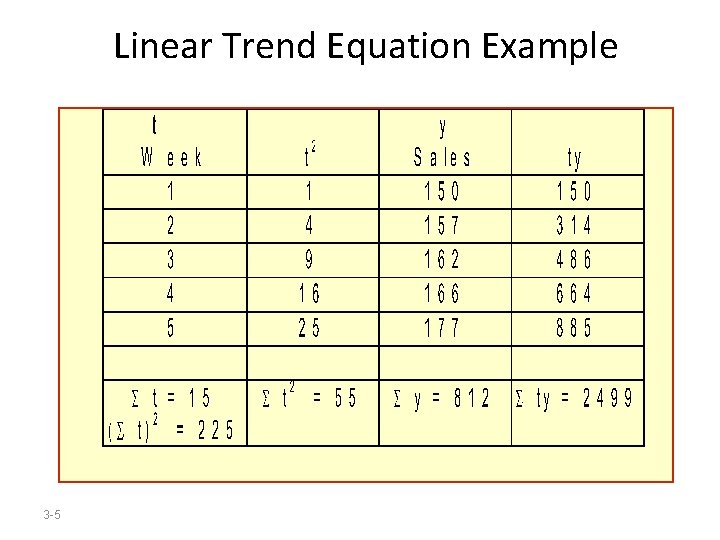
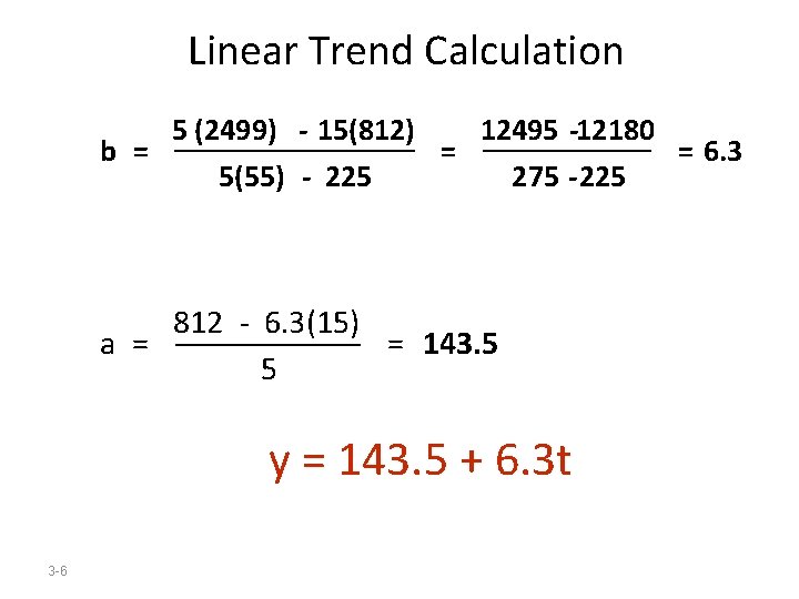
Calculating a and b n (ty) - t y b = 2 2 n t - ( t) y - b t a = n 3 -4

Linear Trend Equation Example 3 -5

Linear Trend Calculation b = 5 (2499) - 15(812) 5(55) - 225 = 12495 -12180 275 -225 812 - 6. 3(15) a = = 143. 5 5 y = 143. 5 + 6. 3 t 3 -6 = 6. 3

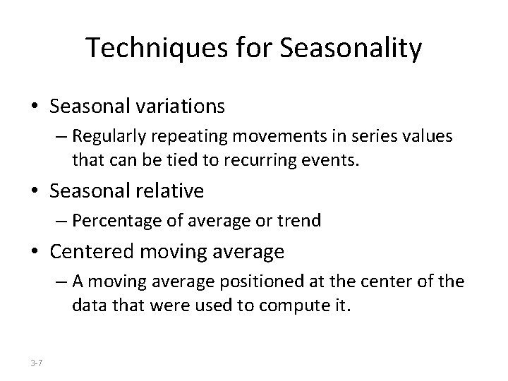
Techniques for Seasonality • Seasonal variations – Regularly repeating movements in series values that can be tied to recurring events. • Seasonal relative – Percentage of average or trend • Centered moving average – A moving average positioned at the center of the data that were used to compute it. 3 -7

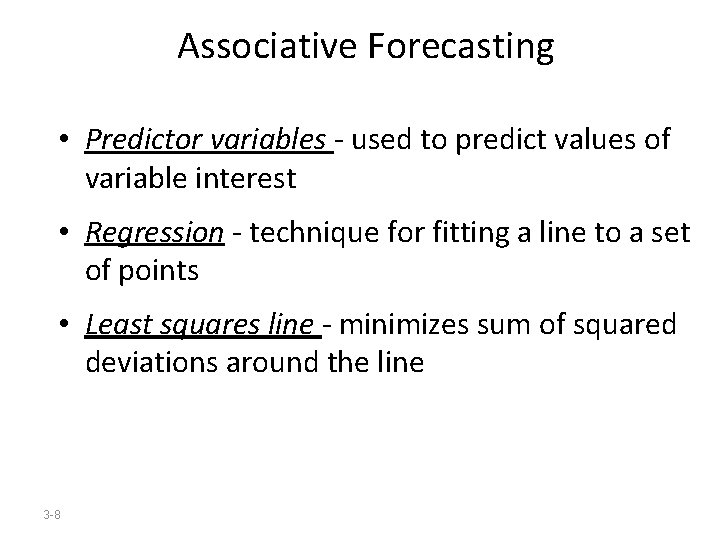
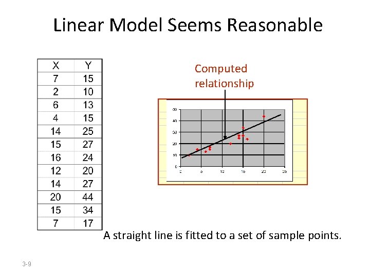
Associative Forecasting • Predictor variables - used to predict values of variable interest • Regression - technique for fitting a line to a set of points • Least squares line - minimizes sum of squared deviations around the line 3 -8

Linear Model Seems Reasonable Computed relationship A straight line is fitted to a set of sample points. 3 -9

Linear Regression Assumptions • Variations around the line are random • Deviations around the line normally distributed • Predictions are being made only within the range of observed values • For best results: – Always plot the data to verify linearity – Check for data being time-dependent – Small correlation may imply that other variables are important 3 -10

A Good Forecast ¨ Has a small error ¨ Error = Demand - Forecast

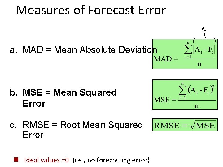
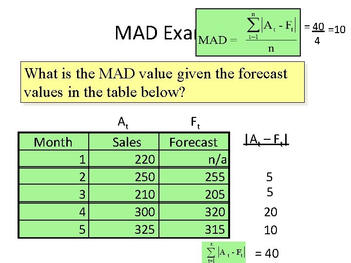
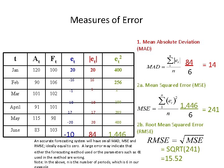
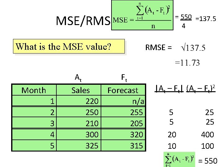
Measures of Forecast Error et a. MAD = Mean Absolute Deviation b. MSE = Mean Squared Error c. RMSE = Root Mean Squared Error n Ideal values =0 (i. e. , no forecasting error)

= 40 =10 4 MAD Example What is the MAD value given the forecast values in the table below? At Month 1 2 3 4 5 Ft Sales Forecast 220 n/a 250 255 210 205 300 325 315 |At – Ft| 5 5 20 10 = 40

Measures of Error 1. Mean Absolute Deviation (MAD) t At Ft et |et| e t 2 Jan 120 100 20 20 400 Feb 90 106 -16 16 -1 1 1 -10 10 100 17 17 289 -20 20 400 -10 84 1, 446 Mar April May June 101 91 115 83 102 101 98 103 256 84 6 = 14 2 a. Mean Squared Error (MSE) 1, 446 = 241 6 2 b. Root Mean Squared Error (RMSE) An accurate forecasting system will have small MAD, MSE and RMSE; ideally equal to zero. A large error may indicate that either the forecasting method used or the parameters such as α used in the method are wrong. Note: In the above, n is the number of periods, which is 6 in our = SQRT(241) =15. 52

= 550 =137. 5 4 MSE/RMSE Example What is the MSE value? RMSE = √ 137. 5 =11. 73 At Month 1 2 3 4 5 Ft Sales Forecast 220 n/a 250 255 210 205 300 325 315 |At – Ft| (At – Ft)2 5 5 20 10 25 25 400 100 = 550

Controlling the Forecast • Control chart – A visual tool for monitoring forecast errors – Used to detect non-randomness in errors • Forecasting errors are in control if – All errors are within the control limits – No patterns, such as trends or cycles, are present 3 -16

Sources of Forecast errors • Model may be inadequate • Irregular variations • Incorrect use of forecasting technique 3 -17

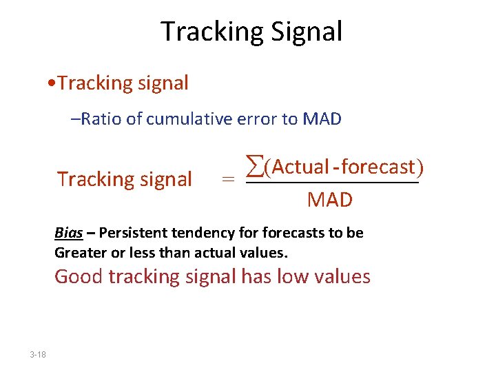
Tracking Signal • Tracking signal –Ratio of cumulative error to MAD Tracking signal (Actual -forecast) = MAD Bias – Persistent tendency forecasts to be Greater or less than actual values. Good tracking signal has low values 3 -18

Choosing a Forecasting Technique • No single technique works in every situation • Two most important factors – Cost – Accuracy • Other factors include the availability of: – Historical data – Computers – Time needed to gather and analyze the data – Forecast horizon 3 -19

To Use a Forecasting Method • Collect historical data • Select a model – Moving average methods • Select n (number of periods) • For weighted moving average: select weights – Exponential smoothing • Selections should produce a good forecast …