Recent developments and perspectives in meteorological data assimilation

Recent developments and perspectives in meteorological data assimilation Jean Pailleux (Météo-France /CNRM / Toulouse) jean. pailleux@meteo. fr Presentation based mainly on experience and work of the NWP teams in Toulouse (Meteo-France) and Reading (ECMWF). Special thanks to the assimilation people of these two teams NWP = Numerical Weather Prediction

Recent developments and perspectives in meteorological data assimilation jean. pailleux@meteo. fr • • • 1. Estimation theory and data assimilation problems. 2. The algorithmic evolution of assimilation in NWP. 3. More and more observation variety for met models. 4. From NWP to ocean, climate, chemistry assimilation 5. Probalistic approach of model forecasting through initial state uncertainties (analysis errors). • 6. Some conclusions on the specific aspects of the atmosphere.

DATA ASSIMILATION (OBJECTIVE ANALYSIS) • Determination of initial conditions for a model, or…. • Estimation from all the available pieces of information (mainly the observations) of the atmospheric state which is necessary to run a NWP model.

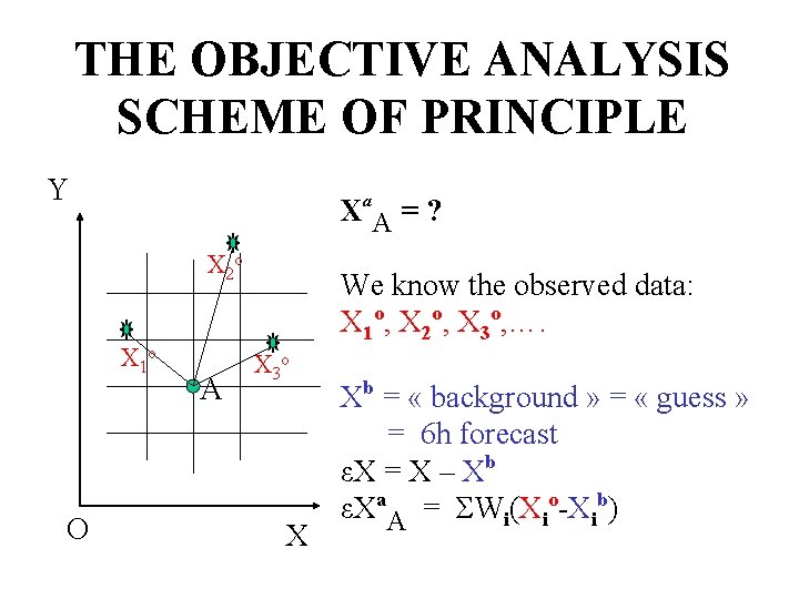
THE OBJECTIVE ANALYSIS SCHEME OF PRINCIPLE Y Xa. A = ? X 2 o X 1 o O A We know the observed data: X 1 o, X 2 o, X 3 o, …. X 3 o X Xb = « background » = « guess » = 6 h forecast εX = X – Xb εXa. A = ΣWi(Xio-Xib)

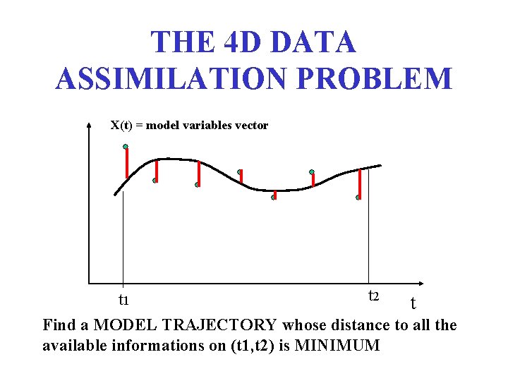
THE 4 D DATA ASSIMILATION PROBLEM X(t) = model variables vector t 2 t 1 t Find a MODEL TRAJECTORY whose distance to all the available informations on (t 1, t 2) is MINIMUM

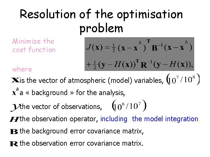
Resolution of the optimisation problem Minimize the cost function where is the vector of atmospheric (model) variables, a « background » for the analysis, the vector of observations, the observation operator, including the model integration, the background error covariance matrix, the observation error covariance matrix.

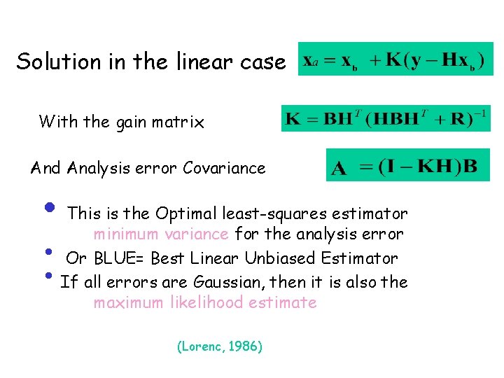
Solution in the linear case With the gain matrix And Analysis error Covariance • This is the Optimal least-squares estimator • • minimum variance for the analysis error Or BLUE= Best Linear Unbiased Estimator If all errors are Gaussian, then it is also the maximum likelihood estimate (Lorenc, 1986)

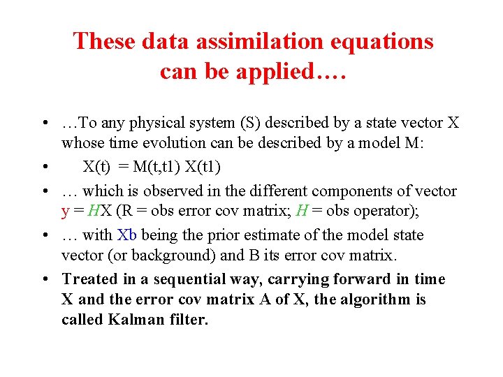
These data assimilation equations can be applied…. • …To any physical system (S) described by a state vector X whose time evolution can be described by a model M: • X(t) = M(t, t 1) X(t 1) • … which is observed in the different components of vector y = HX (R = obs error cov matrix; H = obs operator); • … with Xb being the prior estimate of the model state vector (or background) and B its error cov matrix. • Treated in a sequential way, carrying forward in time X and the error cov matrix A of X, the algorithm is called Kalman filter.

THE OBJECTIVE ANALYSIS SCHEME OF PRINCIPLE Y Xa. A = ? X 2 o X 1 o O A We know the observed data: X 1 o, X 2 o, X 3 o, …. X 3 o X Xb = « background » = « guess » = 6 h forecast εX = X – Xb εXa. A = ΣWi(Xio-Xib)

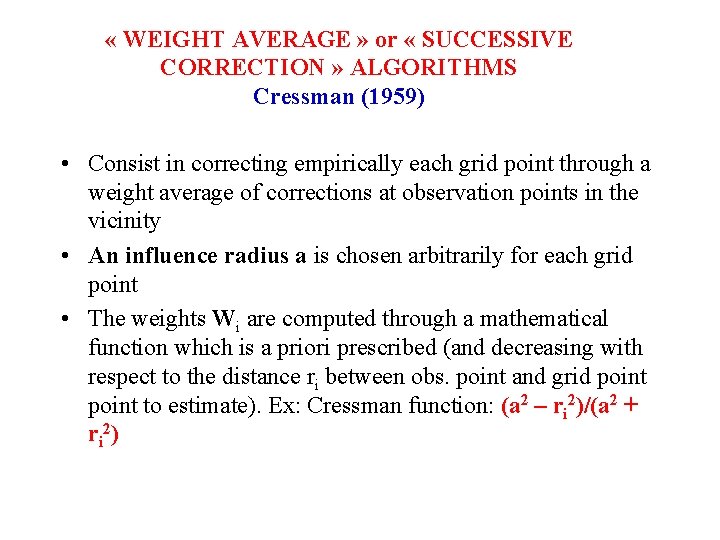
« WEIGHT AVERAGE » or « SUCCESSIVE CORRECTION » ALGORITHMS Cressman (1959) • Consist in correcting empirically each grid point through a weight average of corrections at observation points in the vicinity • An influence radius a is chosen arbitrarily for each grid point • The weights Wi are computed through a mathematical function which is a priori prescribed (and decreasing with respect to the distance ri between obs. point and grid point to estimate). Ex: Cressman function: (a 2 – ri 2)/(a 2 + ri 2)

THE OBJECTIVE ANALYSIS SCHEME OF PRINCIPLE Y Xa. A = ? X 2 o X 1 o O A We know the observed data: X 1 o, X 2 o, X 3 o, …. X 3 o X Xb = « background » = « guess » = 6 h forecast εX = X – Xb εXa. A = ΣWi(Xio-Xib)

OPTIMUM INTERPOLATION Gandin (1963) • The weights Wi are coming out from the resolution of a linear system of equations based on the covariance matrix of the departures « Obs-Background » at the obs. points (subset of the matrix noted (H. B. Ht + R) before) • The space statistical structure of background errors and observation errors has to be modelled (and evaluated a priori): space autocorrelation functions; structure functions. • When several observation types are introduced in the estimation, the scheme is called « multivariate optimum interpolation »

THE OBJECTIVE ANALYSIS SCHEME OF PRINCIPLE Y Xa. A = ? X 2 o X 1 o O A We know the observed data: X 1 o, X 2 o, X 3 o, …. X 3 o X Xb = « background » = « guess » = 6 h forecast εX = X – Xb εXa. A = ΣWi(Xio-Xib)

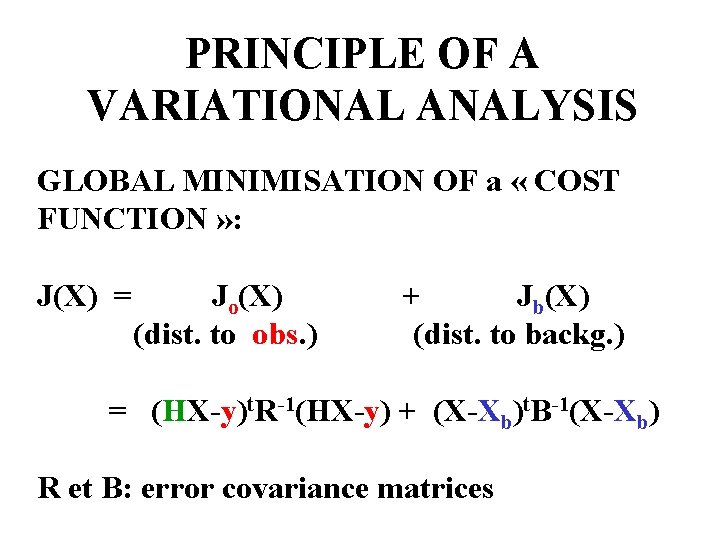
PRINCIPLE OF A VARIATIONAL ANALYSIS GLOBAL MINIMISATION OF a « COST FUNCTION » : J(X) = Jo(X) + Jb(X) (dist. to obs. ) (dist. to backg. ) = (HX-y)t. R-1(HX-y) + (X-Xb)t. B-1(X-Xb) R et B: error covariance matrices

EQUIVALENCE between variational analysis and optimum interpolation • According to the estimation theory there is a mathematical equivalence between the variational formulation (3 D) and the optimum interpolation producing analyses at a given time t… • …If some conditions are met!… such as « using the same observationsfor both algorithms »

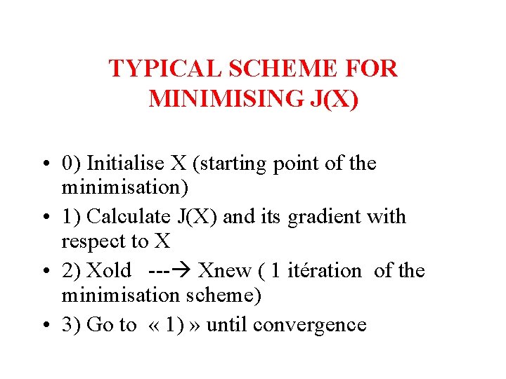
TYPICAL SCHEME FOR MINIMISING J(X) • 0) Initialise X (starting point of the minimisation) • 1) Calculate J(X) and its gradient with respect to X • 2) Xold --- Xnew ( 1 itération of the minimisation scheme) • 3) Go to « 1) » until convergence

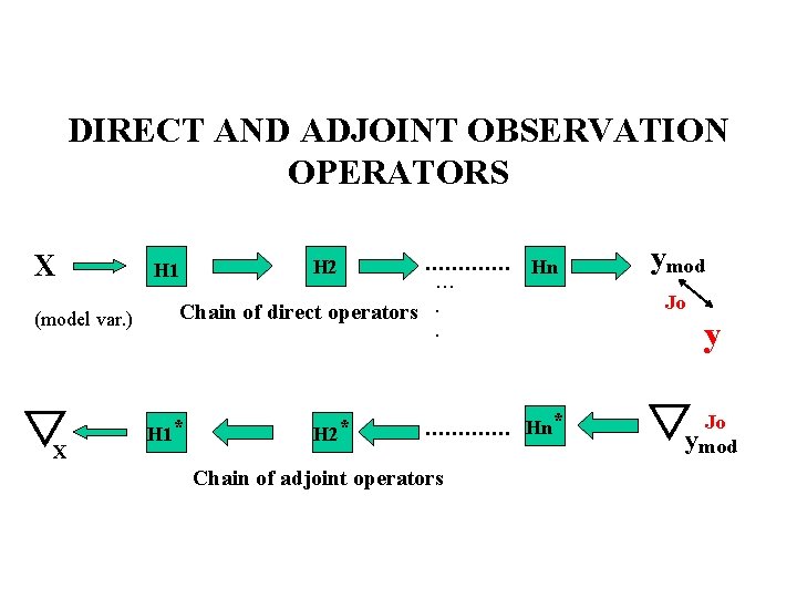
DIRECT AND ADJOINT OBSERVATION OPERATORS X (model var. ) X …………. … Chain of direct operators. . H 1* H 2* Hn …………. Hn* Chain of adjoint operators ymod Jo ymod

3 D-VAR vs OPTIMUM INTERPOLATION • A 3 D Variational analysis (3 D-VAR) guarantees a better space consistency of analysed meteorological fields • Improved possibilities for observation use • 3 D-VAR is an algorithmic step towards 4 DVAR (4 D Variational assimilation)

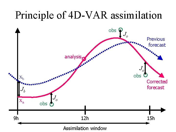
Principle of 4 D-VAR assimilation obs Jo Previous forecast analysis Jo obs xb Jb xa 9 h obs Corrected forecast Jo 12 h Assimilation window 15 h

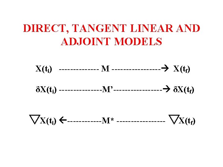
DIRECT, TANGENT LINEAR AND ADJOINT MODELS X(ti) ------- M --------- X(tf) δX(ti) --------M’--------- δX(tf) X(ti) ------M* --------- X(tf)

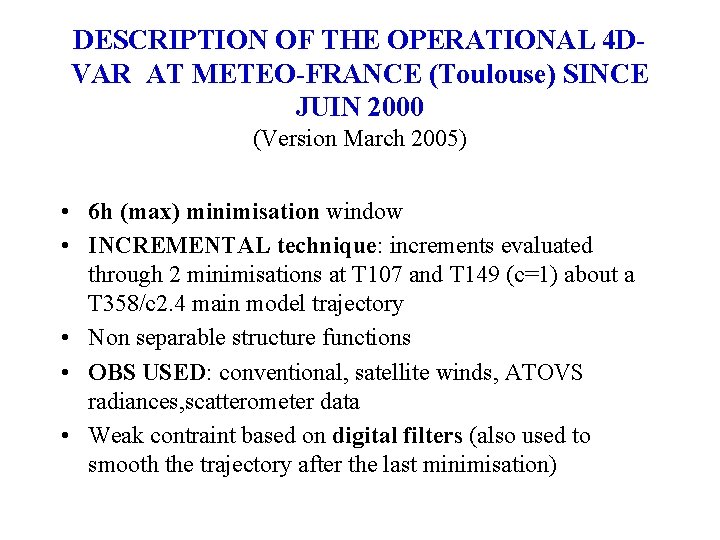
DESCRIPTION OF THE OPERATIONAL 4 DVAR AT METEO-FRANCE (Toulouse) SINCE JUIN 2000 (Version March 2005) • 6 h (max) minimisation window • INCREMENTAL technique: increments evaluated through 2 minimisations at T 107 and T 149 (c=1) about a T 358/c 2. 4 main model trajectory • Non separable structure functions • OBS USED: conventional, satellite winds, ATOVS radiances, scatterometer data • Weak contraint based on digital filters (also used to smooth the trajectory after the last minimisation)

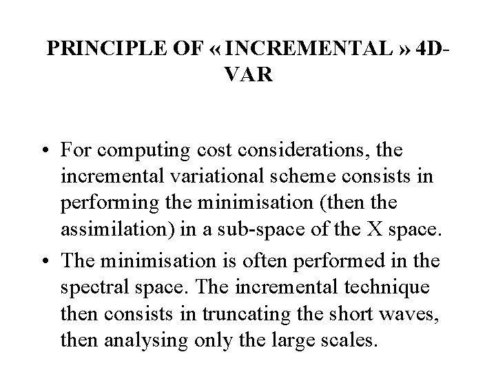
PRINCIPLE OF « INCREMENTAL » 4 DVAR • For computing cost considerations, the incremental variational scheme consists in performing the minimisation (then the assimilation) in a sub-space of the X space. • The minimisation is often performed in the spectral space. The incremental technique then consists in truncating the short waves, then analysing only the large scales.

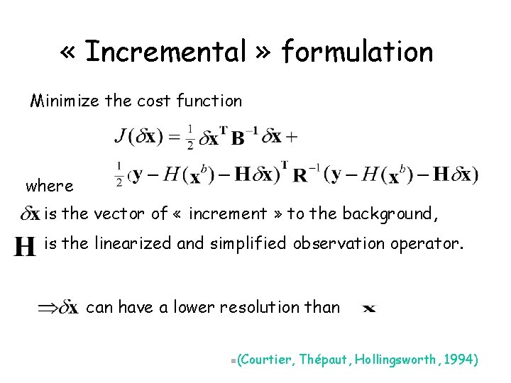
« Incremental » formulation Minimize the cost function where is the vector of « increment » to the background, is the linearized and simplified observation operator. can have a lower resolution than n(Courtier, Thépaut, Hollingsworth, 1994)

Recent developments and perspectives in meteorological data assimilation jean. pailleux@meteo. fr • • • 1. Estimation theory and data assimilation problems. 2. The algorithmic evolution of assimilation in NWP. 3. More and more observation variety for met models. 4. From NWP to ocean, climate, chemistry assimilation 5. Probalistic approach of model forecasting through initial state uncertainties (analysis errors). • 6. Some conclusions on the specific aspects of the atmosphere.

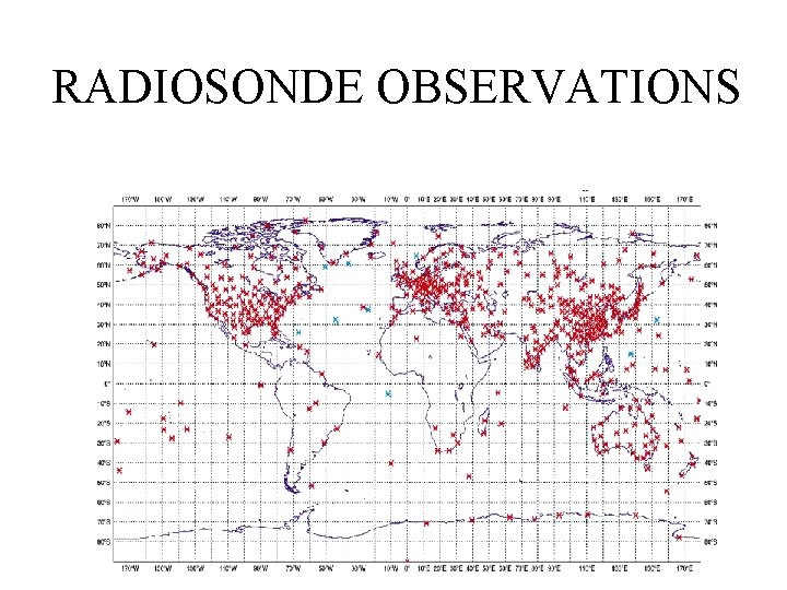
RADIOSONDE OBSERVATIONS

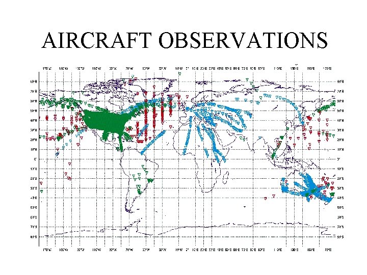
AIRCRAFT OBSERVATIONS

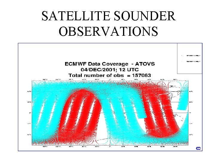
SATELLITE SOUNDER OBSERVATIONS

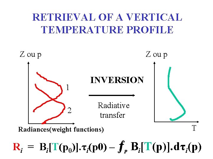
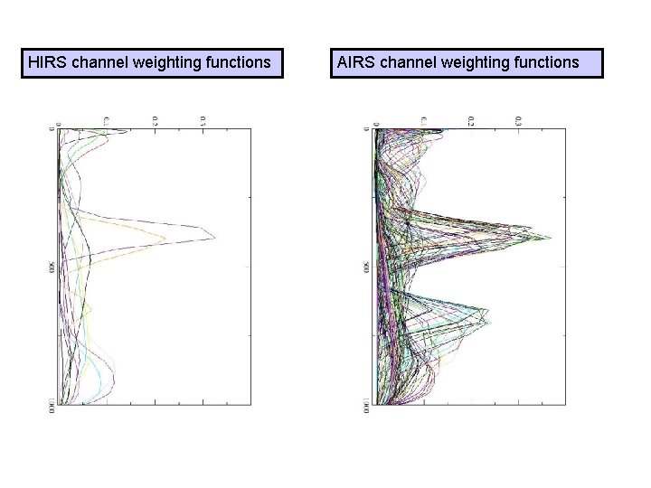
RETRIEVAL OF A VERTICAL TEMPERATURE PROFILE Z ou p 1 2 INVERSION Radiative transfer Radiances(weight functions) T Ri = Bi[T(p 0)]. τi(p 0) – ƒp Bi[T(p)]. dτi(p)

HIRS channel weighting functions AIRS channel weighting functions

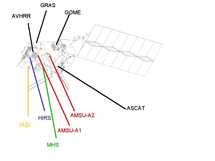
GRAS GOME AVHRR ASCAT AMSU-A 2 HIRS IASI AMSU-A 1 MHS

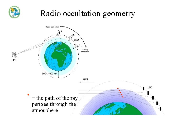
Radio occultation geometry = the path of the ray perigee through the atmosphere

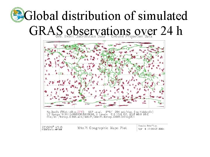
Global distribution of simulated GRAS observations over 24 h

Recent developments and perspectives in meteorological data assimilation jean. pailleux@meteo. fr • • • 1. Estimation theory and data assimilation problems. 2. The algorithmic evolution of assimilation in NWP. 3. More and more observation variety for met models. 4. From NWP to ocean, climate, chemistry assimilation 5. Probalistic approach of model forecasting through initial state uncertainties (analysis errors). • 6. Some conclusions on the specific aspects of the atmosphere.

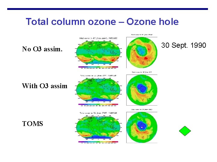
Data assimilation and atmospheric chemistry • More and more atmospheric chemical species (O 3, Nox, …) are observed and assimilated into chemical models. • Some operational NWP models (e. g. ECMWF) are treating ozone and assimilating ozone data.

Total column ozone – Ozone hole No O 3 assim. With O 3 assim TOMS 30 Sept. 1990

Data assimilation and ocean modelling • Data assimilation is operational in several oceanographic centres • Observations: SST (Sea Surface Temperature), SSH (Sea Surface Height – altimeter), temperature and salinity profiles, etc…

Data assimilation and climate modelling • Coupled atmospheric and ocean systems used for simulating the evolution of the climate • Climate studies relies more enad more on « re-analyses » performed with simplified versions of NWP data assimilation systems (e; g; : http: //www. ecmwf. int/research/era/ to study ERA 40)

Recent developments and perspectives in meteorological data assimilation jean. pailleux@meteo. fr • • • 1. Estimation theory and data assimilation problems. 2. The algorithmic evolution of assimilation in NWP. 3. More and more observation variety for met models. 4. From NWP to ocean, climate, chemistry assimilation 5. Probalistic approach of model forecasting through initial state uncertainties (analysis errors). • 6. Some conclusions on the specific aspects of the atmosphere.

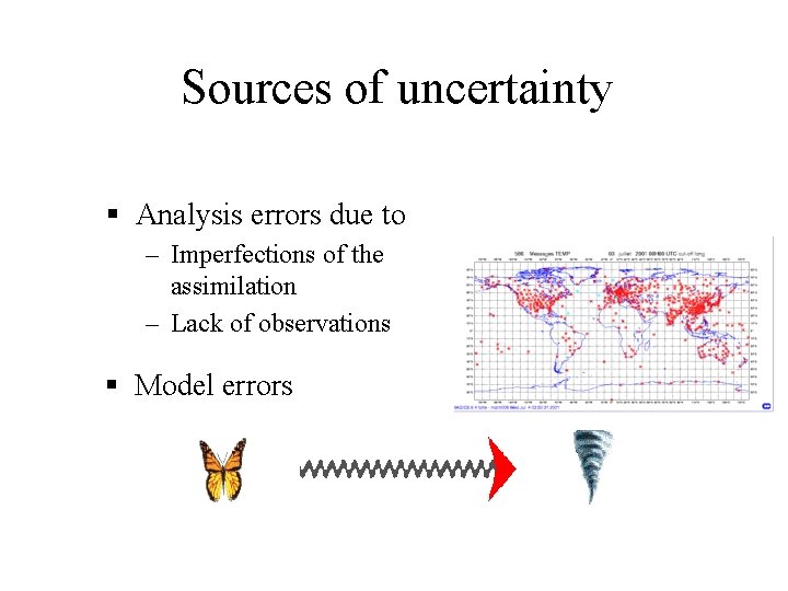
Sources of uncertainty § Analysis errors due to – Imperfections of the assimilation – Lack of observations § Model errors

How can we take into account the initial uncertainty • Analysis perturbations to sample the more unstable modes – Based on the computation of the more unstable modes – Perturbations consistent with the analysis error estimate – Méthod : singular vectors, • Sampling of the model uncertainty – Perturbation of some physical parameters… – Etc…

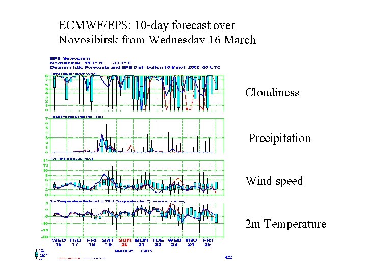
ECMWF/EPS: 10 -day forecast over Novosibirsk from Wednesday 16 March 00 UTC • Cloudiness Precipitation Wind speed 2 m Temperature

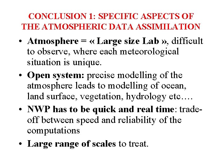
CONCLUSION 1: SPECIFIC ASPECTS OF THE ATMOSPHERIC DATA ASSIMILATION • Atmosphere = « Large size Lab » , difficult to observe, where each meteorological situation is unique. • Open system: precise modelling of the atmosphere leads to modelling of ocean, land surface, vegetation, hydrology etc…. • NWP has to be quick and real time: tradeoff between speed and reliability of the computations • Large range of scales to treat.

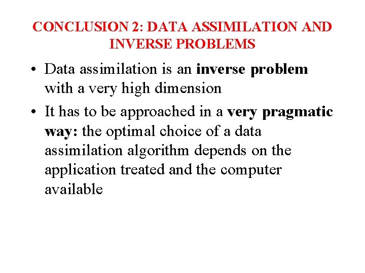
CONCLUSION 2: DATA ASSIMILATION AND INVERSE PROBLEMS • Data assimilation is an inverse problem with a very high dimension • It has to be approached in a very pragmatic way: the optimal choice of a data assimilation algorithm depends on the application treated and the computer available

RESERVE For questions Not to be shown

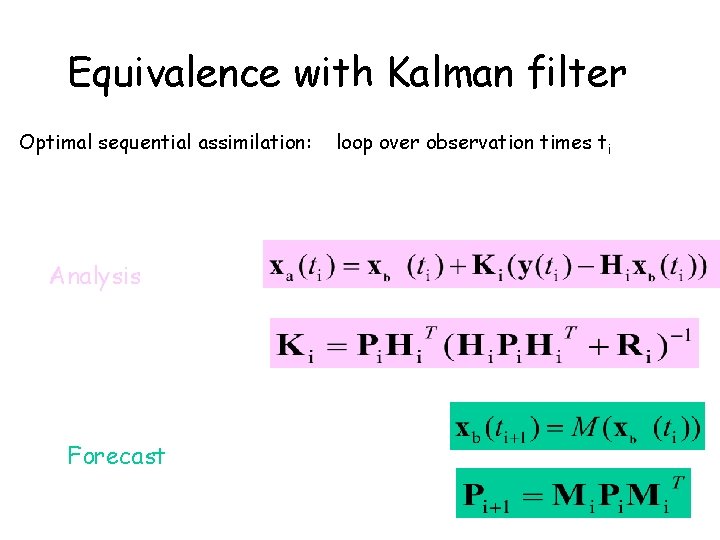
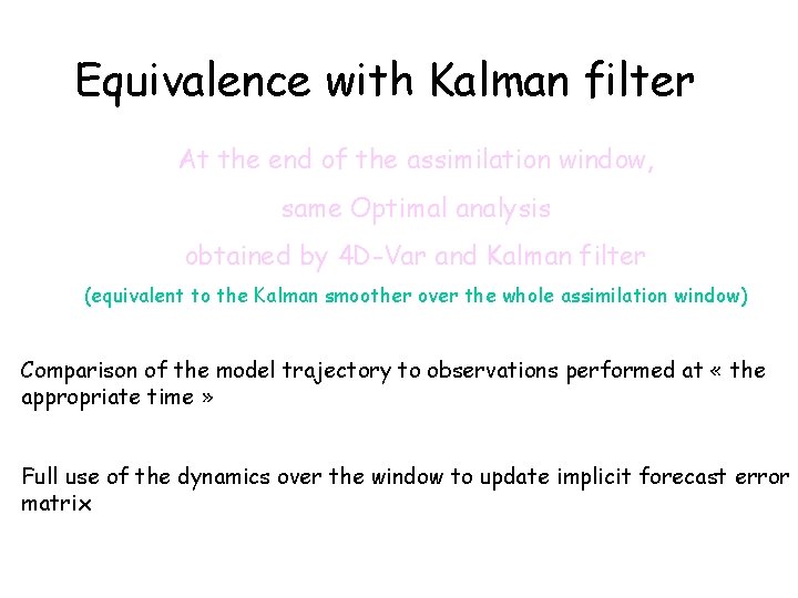
Equivalence with Kalman filter Optimal sequential assimilation: Analysis Forecast loop over observation times ti

Equivalence with Kalman filter At the end of the assimilation window, same Optimal analysis obtained by 4 D-Var and Kalman filter (equivalent to the Kalman smoother over the whole assimilation window) Comparison of the model trajectory to observations performed at « the appropriate time » Full use of the dynamics over the window to update implicit forecast error matrix

Properties of Variational methods Can be extended to non-Gaussian errors: Var-QC (Lorenc, Andersson) Can use a wide range of observations including those with a complex link to atmospheric variables (eg radiances, Andersson et al, 1994) Efficient use of asynoptic data (Järvinen, Andersson)

Data assimilation • Problems to consider in an operational analysis : - nature and quality of the different observations - Quality control - Taking into account the information coming from the past - Preserve the atmosphere balance and control the waves which are not relevant for modeling

ADM-AEOLUS (space lidar)

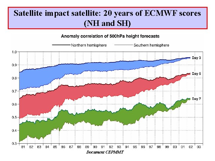
Satellite impact satellite: 20 years of ECMWF scores (NH and SH) Document CEPMMT

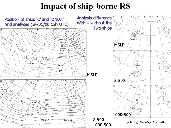
Impact of ship-borne RS Position of ships ‘C’ and ‘ONDA’ And analyses (24/01/90 12 h UTC) Analysis difference With – without the Two ships MSLP Z 500 –– Z 500 - - 1000 -500 (Heming, Met. Mag. 119, 1990)

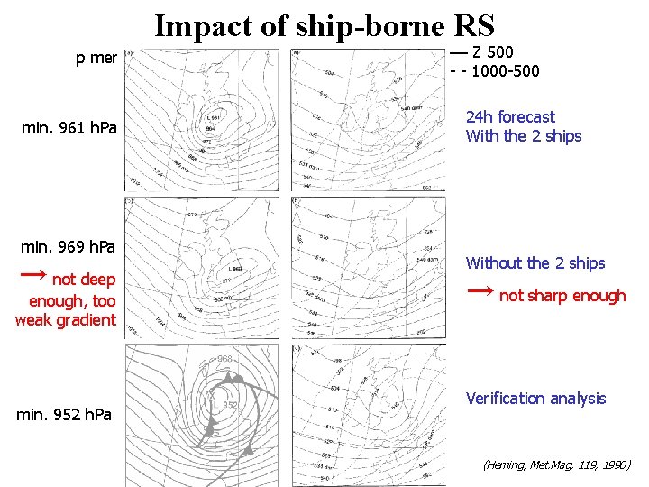
Impact of ship-borne RS p mer min. 961 h. Pa min. 969 h. Pa → not deep enough, too weak gradient min. 952 h. Pa –– Z 500 - - 1000 -500 24 h forecast With the 2 ships Without the 2 ships → not sharp enough Verification analysis (Heming, Met. Mag. 119, 1990)