Ocean Data Assimilation Hao Zuo Earth System Assimilation

Ocean Data Assimilation Hao Zuo Earth System Assimilation Section With input from Magdalena Balmaseda, Kristian Mogensen, Mohamed Dahoui and others DA Training Course 2017: Ocean Data Assimilation 1

Outline of lecture • General remarks Ø Applications of ocean data assimilation Ø Ocean versus Atmosphere DA Ø The Ocean Observing System • An example of Ocean DA: NEMOVAR Ø Ø Ø NEMOVAR general Background co-variances Balance relationships: temperature, salinity, sea level and velocity Altimeter assimilation Bias correction • Ocean analysis system Ø OCEAN 5 operational system Ø Monitoring of OCEAN 5 analysis DA Training Course 2017: Ocean Data Assimilation 2

OCEAN DA: components 1. The blue ocean: ocean dynamics. Ø Primary variables: potential temperature (T), salinity (S) current (U, V) and sea surface height (SSH). Ø Density is a function of T and S though the equation of state. 2. The white ocean: sea-ice. Not covered here Ø Ø Sea ice concentration and thickness. Very few thickness obs Non gaussian errors. Unknown balance relationships 3. The green ocean: biogeochemistry. Not covered DA Training Course 2017: Ocean Data Assimilation 3

Why do we do ocean DA? • Forecasting: initialization of coupled models Ø NWP, monthly, seasonal, decadal. Ø Different depths of the ocean are involved at different time scales Ø Climate resolution (global ~1, 1/4 degrees, … 1/12) • Reconstruct & monitor the ocean (re-analysis) • Monitor/forecast the ocean mesoscale and biochemestry Ø High resolution ocean analysis (regional, ~1/3 -1/9 -1/12 degrees) Ø Defence, commercial applications (oil rigs …), safety and rescue, environmental (algii blooms, spills) DA Training Course 2017: Ocean Data Assimilation 4

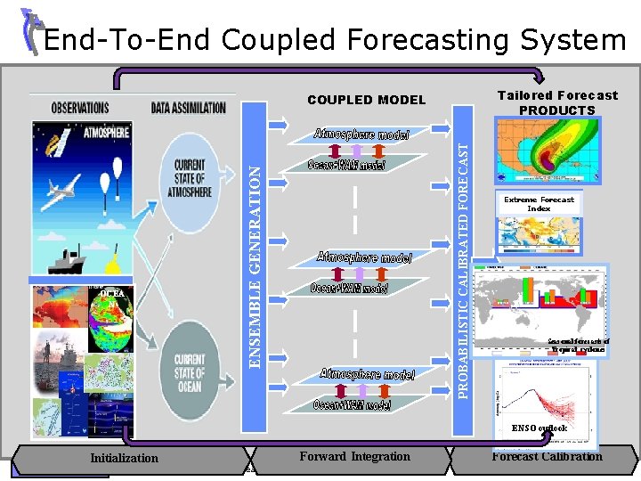
End-To-End Coupled Forecasting System Tailored Forecast PRODUCTS ENSEMBLE GENERATION OCEA N PROBABILISTIC CALIBRATED FORECAST COUPLED MODEL Extreme Forecast Index Seasonal forecasts of Tropical cyclones ENSO outlook Initialization Forward Integration DA Training Course 2017: Ocean Data Assimilation Forecast Calibration 5

Ocean versus Atmosphere: some facts • Spatial/time scales The radius of deformation in the ocean is small (~30 km) compared to the atmosphere (~3000 km). Radius of deformation =c/f where c= speed of gravity waves. In the ocean c~<3 m/s for baroclinic processes. Smaller spatial scales and Longer time scales • The ocean is strongly stratified in the vertical, although deep convection also occurs Density is determined by Temperature and Salinity • The ocean is forced at the surface by the wind/waves, by heating/cooling, and by fresh-water fluxes. Uncertainty in forcing fluxes contributes to uncertainty in model results. • The electromagnetic radiation does not penetrate into the ocean, which makes the deep ocean difficult to observe from satellites. The surface of the ocean can however be observed from space • The ocean has continental boundaries; dealing with them is not trivial in data assimilation DA Training Course 2017: Ocean Data Assimilation 6

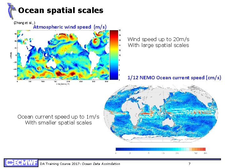
Ocean spatial scales 2 - Ocean Weather (Zhang et al. , ) Atmospheric wind speed (m/s) Wind speed up to 20 m/s With large spatial scales 1/12 NEMO Ocean current speed (cm/s) Ocean current speed up to 1 m/s With smaller spatial scales DA Training Course 2017: Ocean Data Assimilation 7

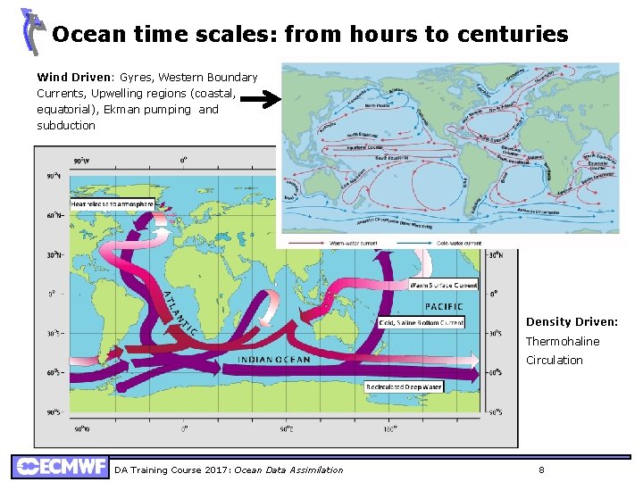
Ocean time scales: from hours to centuries Wind Driven: Gyres, Western Boundary Currents, Upwelling regions (coastal, equatorial), Ekman pumping and subduction Density Driven: Thermohaline Circulation DA Training Course 2017: Ocean Data Assimilation 8

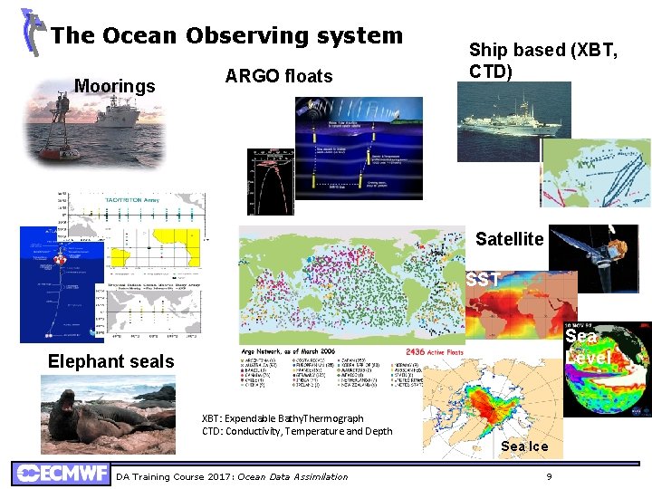
The Ocean Observing system Moorings ARGO floats Ship based (XBT, CTD) Satellite SST Sea Level Elephant seals XBT: Expendable Bathy. Thermograph CTD: Conductivity, Temperature and Depth Sea Ice DA Training Course 2017: Ocean Data Assimilation 9

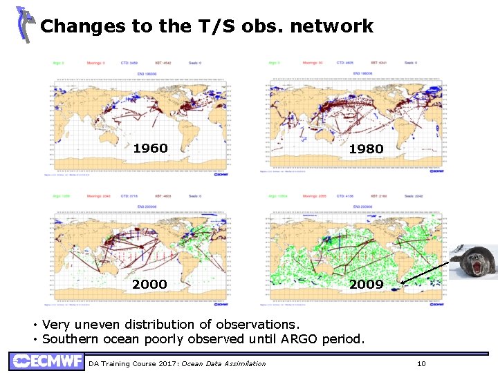
Changes to the T/S obs. network 1960 1980 2009 • Very uneven distribution of observations. • Southern ocean poorly observed until ARGO period. DA Training Course 2017: Ocean Data Assimilation 10

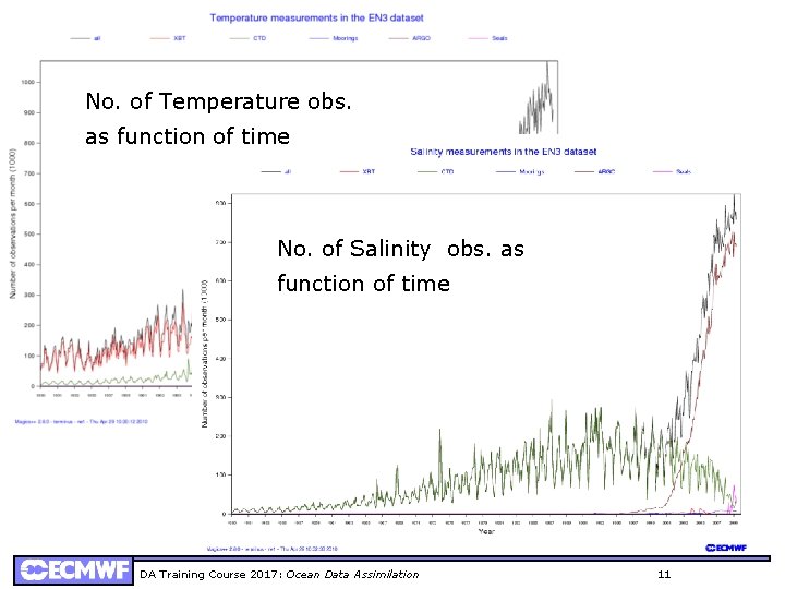
No. of Temperature obs. as function of time No. of Salinity obs. as function of time DA Training Course 2017: Ocean Data Assimilation 11

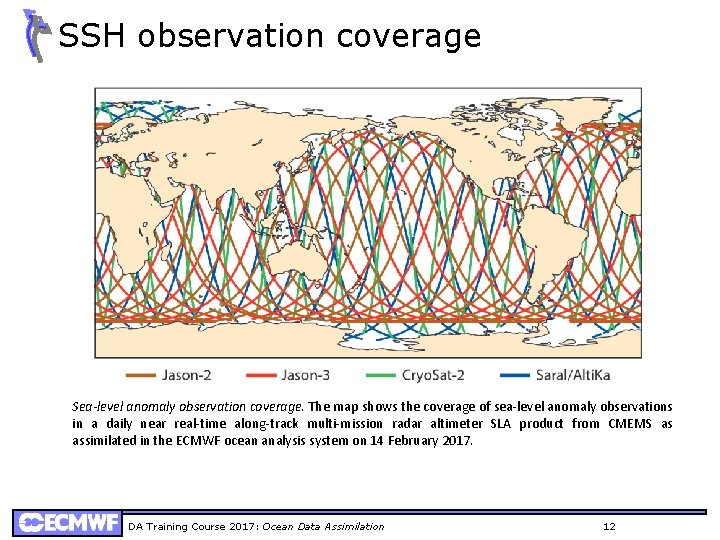
SSH observation coverage Sea-level anomaly observation coverage. The map shows the coverage of sea-level anomaly observations in a daily near real-time along-track multi-mission radar altimeter SLA product from CMEMS as assimilated in the ECMWF ocean analysis system on 14 February 2017. DA Training Course 2017: Ocean Data Assimilation 12

Ocean assimilation systems • DA systems based on optimum interpolation (OI), variational techniques (e. g. 3 D/4 D-Var) or various ensemble Kalman filter based methods. Ø Or various hybrid combinations, just like for the atmospheric systems. • First guess given by an ocean model forced by atmospheric fluxes. • Usually observations are used to modify Temperature (T), Salinity (S) and SSH. No direct assimilation of velocities, but derived via balance relationships. • How to deal with coast lines is not trivial. Ø E. g. we don’t want increments (result of analysis) from the Pacific to propagate to the Atlantic across Panama. • Bias correction is very important for reanalyses applications (see later) DA Training Course 2017: Ocean Data Assimilation 13

NEMOVAR assimilation systems • The “NEMOVAR” assimilation system used in ECMWF. Ø Variational system as a collaborative project among CERFACS, ECMWF, INRIA and the Met Office for assimilation into the NEMO ocean model. o Solves a linearized version of the full non-linear cost function. o Incremental 3 D-Var FGAT running operational, 4 D-Var in research model Ø This system has been adopted by ECMWF and the Met Office for operational ocean data assimilation. Ø Use diffusion operators for background correlation model (not discussed here). Ø Background errors are correlated between different variables through balance operator • To avoid initialization shock increments are typically applied via Incremental Analysis Update (IAU) which applies the increments as a forcing term over a period of time. DA Training Course 2017: Ocean Data Assimilation 14

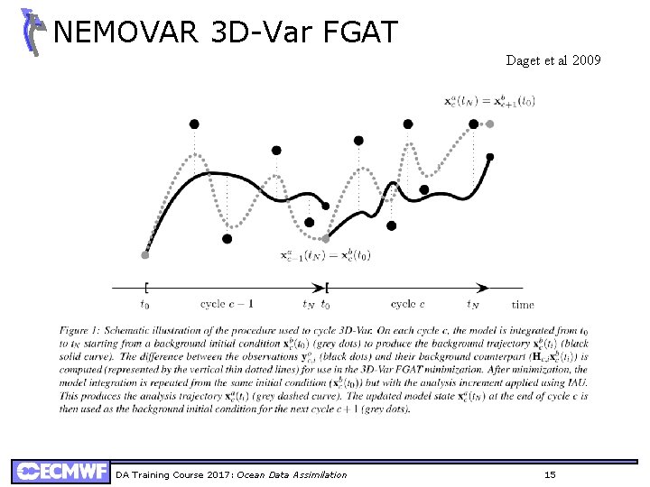
NEMOVAR 3 D-Var FGAT Daget et al 2009 DA Training Course 2017: Ocean Data Assimilation 15

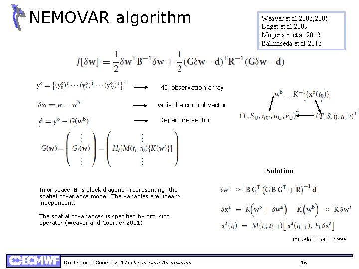
NEMOVAR algorithm Weaver et al 2003, 2005 Daget et al 2009 Mogensen et al 2012 Balmaseda et al 2013 4 D observation array w is the control vector Departure vector Solution In w space, B is block diagonal, representing the spatial covariance model. The variables are linearly independent. The spatial covariances is specified by diffusion operator (Weaver and Courtier 2001) IAU, Bloom et al 1996 DA Training Course 2017: Ocean Data Assimilation 16

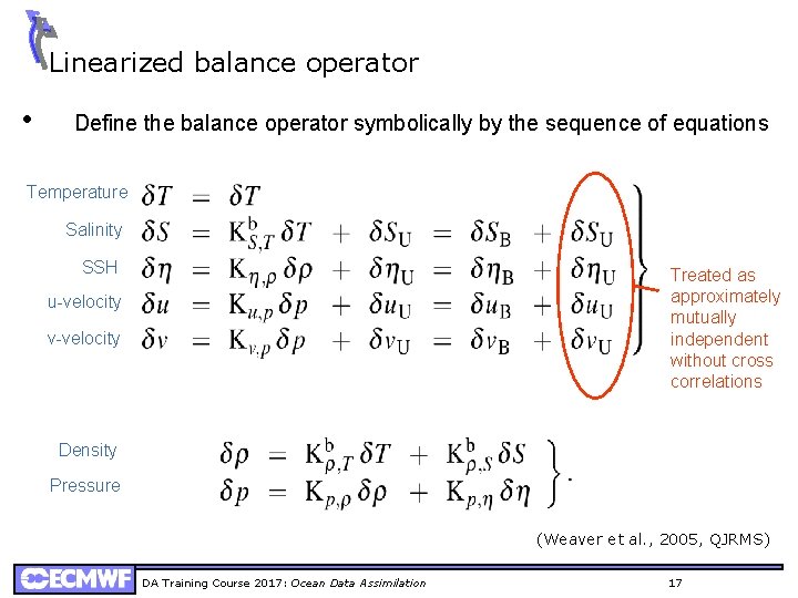
Linearized balance operator • Define the balance operator symbolically by the sequence of equations Temperature Salinity SSH Treated as approximately mutually independent without cross correlations u-velocity v-velocity Density Pressure (Weaver et al. , 2005, QJRMS) DA Training Course 2017: Ocean Data Assimilation 17

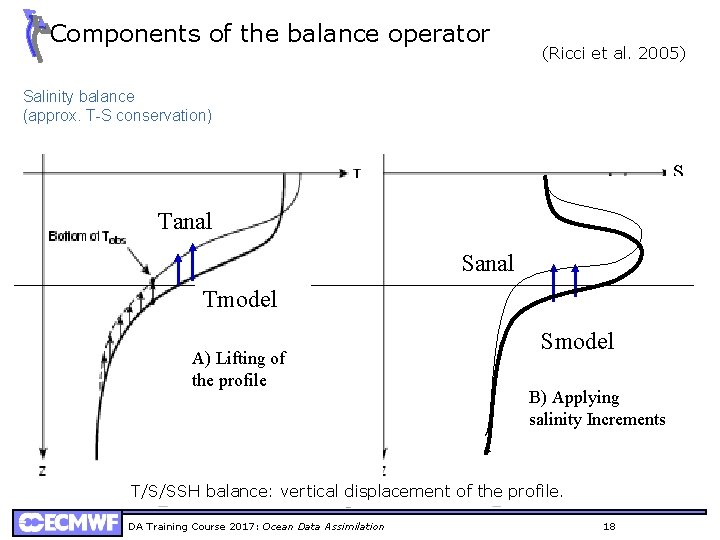
Components of the balance operator (Ricci et al. 2005) Salinity balance (approx. T-S conservation) SSH balance (baroclinic) S Tanal u-velocity balance (geostrophy with β-plane approx. near eq. ) Sanal Tmodel v-velocity (geostrophy, zero at eq. ) A) Lifting of the profile Density (linearized eq. of state) Smodel B) Applying salinity Increments Pressure (hydrostatic approx. ) T/S/SSH balance: vertical displacement of the profile. DA Training Course 2017: Ocean Data Assimilation 18

Background Errors for Ocean DA. • Typical length scales for the applications at ECMWF : Ø ~1 -2 degree at mid latitudes Ø ~15 -20 degrees along the eq. • The background error correlation scales are highly non isotropic to reflect the nature of equatorial waves- Equatorial Kelvin waves which travel rapidly along the equator ~2 m/s but have only a limited meridional scale as they are trapped to the equator. • Complex structures and smaller length scales near coastlines are usually ignored. • The background errors include some (but not all) flow dependent aspects. DA Training Course 2017: Ocean Data Assimilation 19

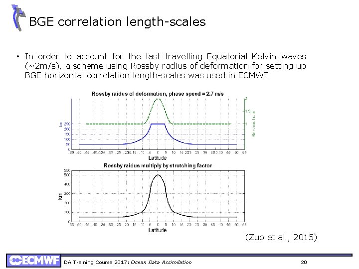
BGE correlation length-scales • In order to account for the fast travelling Equatorial Kelvin waves (~2 m/s), a scheme using Rossby radius of deformation for setting up BGE horizontal correlation length-scales was used in ECMWF. (Zuo et al. , 2015) DA Training Course 2017: Ocean Data Assimilation 20

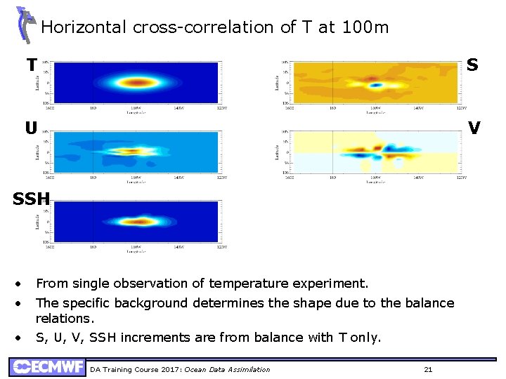
Horizontal cross-correlation of T at 100 m T S U V SSH • • From single observation of temperature experiment. • S, U, V, SSH increments are from balance with T only. The specific background determines the shape due to the balance relations. DA Training Course 2017: Ocean Data Assimilation 21

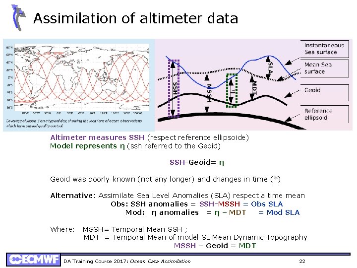
Assimilation of altimeter data Altimeter measures SSH (respect reference ellipsoide) Model represents η (ssh referred to the Geoid) SSH-Geoid= η Geoid was poorly known (not any longer) and changes in time (*) Alternative: Assimilate Sea Level Anomalies (SLA) respect a time mean Obs: SSH anomalies = SSH-MSSH = Obs SLA Mod: η anomalies = η – MDT = Mod SLA Where: MSSH= Temporal Mean SSH ; MDT = Temporal Mean of model SL Mean Dynamic Topography MSSH – Geoid = MDT DA Training Course 2017: Ocean Data Assimilation 22

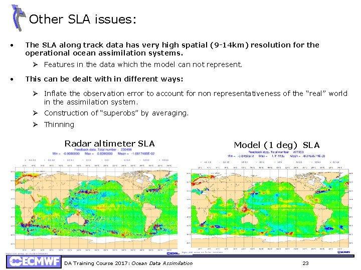
Other SLA issues: • The SLA along track data has very high spatial (9 -14 km) resolution for the operational ocean assimilation systems. Ø Features in the data which the model can not represent. • This can be dealt with in different ways: Ø Inflate the observation error to account for non representativeness of the “real” world in the assimilation system. Ø Construction of “superobs” by averaging. Ø Thinning Radar altimeter SLA DA Training Course 2017: Ocean Data Assimilation Model (1 deg) SLA 23

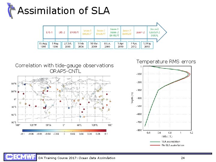
Assimilation of SLA Correlation with tide-gauge observations ORAP 5 -CNTL DA Training Course 2017: Ocean Data Assimilation Temperature RMS errors 24

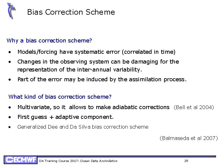
Bias Correction Scheme Why a bias correction scheme? • Models/forcing have systematic error (correlated in time) • Changes in the observing system can be damaging for the representation of the inter-annual variability. • Part of the error may be induced by the assimilation process. What kind of bias correction scheme? • Multivariate, so it allows to make adiabatic corrections (Bell et al 2004) • First guess + adaptive component. • Generalized Dee and Da Silva bias correction scheme (Balmaseda et al 2007) DA Training Course 2017: Ocean Data Assimilation 25

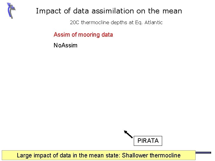
Impact of data assimilation on the mean 20 C thermocline depths at Eq. Atlantic Assim of mooring data No. Assim PIRATA Large impact of. Course data 2017: in Ocean the Data mean state: Shallower thermocline 26 DA Training Assimilation

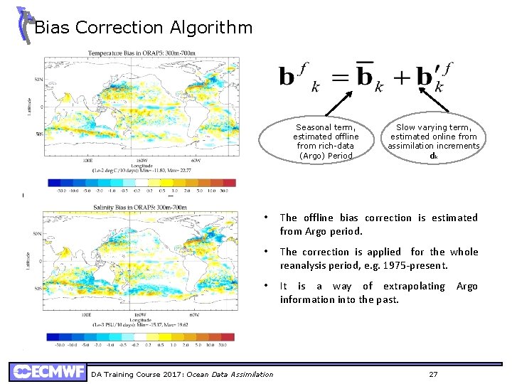
Bias Correction Algorithm Seasonal term, estimated offline from rich-data (Argo) Period Slow varying term, estimated online from assimilation increments dk • The offline bias correction is estimated from Argo period. • The correction is applied for the whole reanalysis period, e. g. 1975 -present. • It is a way of extrapolating Argo information into the past. DA Training Course 2017: Ocean Data Assimilation 27

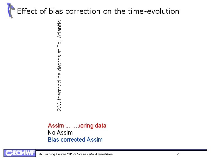
20 C thermocline depths at Eq. Atlantic Effect of bias correction on the time-evolution Assim of mooring data No Assim Bias corrected Assim DA Training Course 2017: Ocean Data Assimilation 28

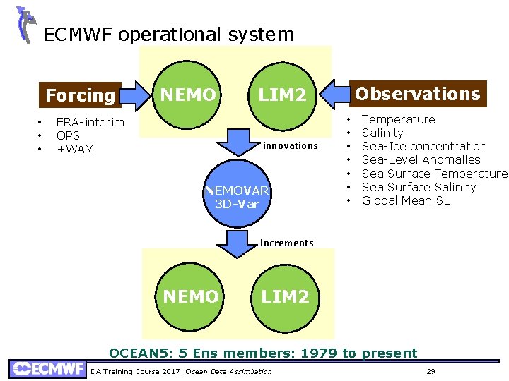
ECMWF operational system Forcing • • • NEMO ERA-interim OPS +WAM Observations LIM 2 innovations NEMOVAR 3 D-Var • • Temperature Salinity Sea-Ice concentration Sea-Level Anomalies Sea Surface Temperature Sea Surface Salinity Global Mean SL increments NEMO LIM 2 OCEAN 5: 5 Ens members: 1979 to present DA Training Course 2017: Ocean Data Assimilation 29

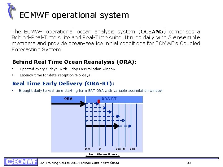
ECMWF operational system The ECMWF operational ocean analysis system (OCEAN 5) comprises a Behind-Real-Time suite and Real-Time suite. It runs daily with 5 ensemble members and provide ocean-sea ice initial conditions for ECMWF’s Coupled Forecasting System. Behind Real Time Ocean Reanalysis (ORA): • Updated every 5 days, with 5 days assimilation window • Latency time for data reception 3 -6 days Real Time Early Delivery (ORA-RT): • Brought daily to real time starting form BRT ORA with variable assimilation window ORA-RT D-m D D-m+N D+N Assim Window N days DA Training Course 2017: Ocean Data Assimilation 30

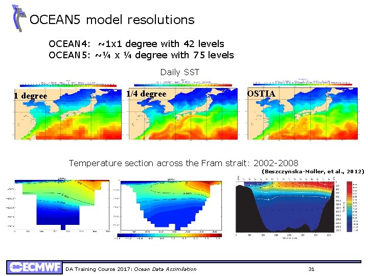
OCEAN 5 model resolutions OCEAN 4: ~1 x 1 degree with 42 levels OCEAN 5: ~¼ x ¼ degree with 75 levels Daily SST 1 degree 1/4 degree OSTIA Temperature section across the Fram strait: 2002 -2008 (Beszczynska-Moller, et al. , 2012) DA Training Course 2017: Ocean Data Assimilation 31

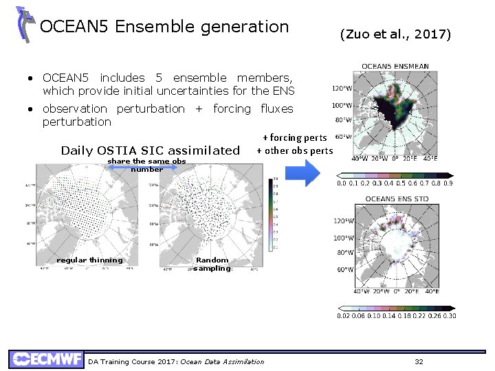
OCEAN 5 Ensemble generation (Zuo et al. , 2017) • OCEAN 5 includes 5 ensemble members, which provide initial uncertainties for the ENS • observation perturbation + forcing fluxes perturbation + forcing perts Daily OSTIA SIC assimilated + other obs perts share the same obs number regular thinning Random sampling DA Training Course 2017: Ocean Data Assimilation 32

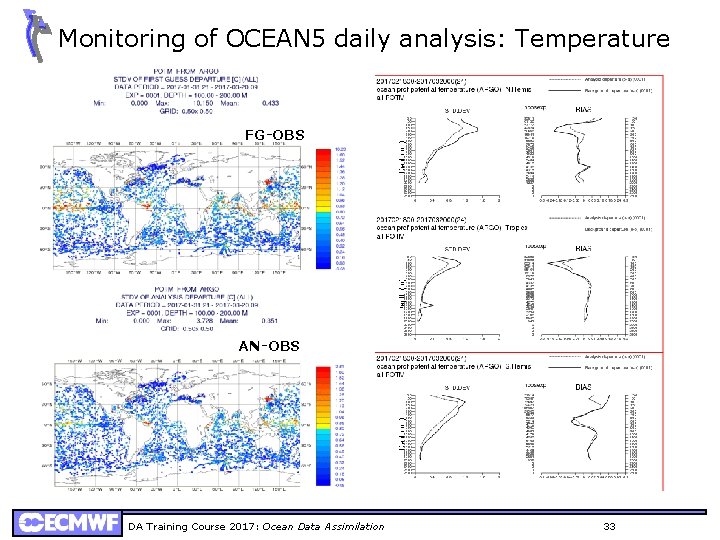
Monitoring of OCEAN 5 daily analysis: Temperature FG-OBS AN-OBS DA Training Course 2017: Ocean Data Assimilation 33

Summary • Data assimilation in the ocean serves a variety of purposes, from climate monitoring to initialization of coupled model forecasts and ocean mesoscale prediction. • This lecture dealt mainly with ocean DA for initialization of coupled forecasts and reanalyses. Global Climate resolution. NEMOVAR as an example. • Compared to the atmosphere, ocean observations are scarce. The main source of information are temperature and salinity profiles (ARGO/moorings/XBTs), sea level from altimeter, SST and SIC from satellite/ships and geoid from gravity missions. • Assimilation of ocean observations reduces the large uncertainty(error) due to the forcing fluxes. It also improves the initialization of seasonal forecasts and decadal forecasts and it can provide useful reconstructions of the ocean climate. • Data assimilation changes the ocean mean state. Therefore, consistent ocean reanalysis requires an explicit treatment of the bias. More generally, we need a methodology that allows the assimilation of different time scales. • Assimilation of Sea-Level data requires consideration: e. g. conversion between SSH and SLA, calculation of MDT, thinning or superob of the SLA observations. DA Training Course 2017: Ocean Data Assimilation 34

Further Readings Ocean Data assimilation • Mogensen, K. , Alonso Balmaseda, M. , & Weaver, A. (2012). The NEMOVAR ocean data assimilation system as implemented in the ECMWF ocean analysis for System 4. Technical Memorandum (Vol. 668). • Weaver, A. T. , Deltel, C. , Machu, É. , Ricci, S. , & Daget, N. (2005). A multivariate balance operator for variational ocean data assimilation. Quarterly Journal of the Royal Meteorological Society, 131(613), 3605– 3625. • Daget, N. , Weaver, A. T. , & Balmaseda, M. A. (2009). Ensemble estimation of background-error variances in a three-dimensional variational data assimilation system for the global ocean. Quarterly Journal of the Royal Meteorological Society, 135(641), 1071– 1094. http: //doi. org/10. 1002/qj. 412 Ocean Reanalysis system • Balmaseda, M. A. , Mogensen, K. , & Weaver, A. T. (2013). Evaluation of the ECMWF ocean reanalysis system ORAS 4. Quarterly Journal of the Royal Meteorological Society, 139(674), 1132– 1161. http: //doi. org/10. 1002/qj. 2063 • Zuo, H. , Balmaseda, M. A. , & Mogensen, K. (2015). The new eddy-permitting ORAP 5 ocean reanalysis: description, evaluation and uncertainties in climate signals. Climate Dynamics. http: //doi. org/10. 1007/s 00382 -015 -2675 -1 DA Training Course 2017: Ocean Data Assimilation 35