CSE 411 Computer Graphics Lecture 10 3 D

CSE 411 Computer Graphics Lecture #10 3 D Object Representations Prepared & Presented by Asst. Prof. Dr. Samsun M. BAŞARICI

Objectives HB Ch. 13 -15 & 23, GVS Ch. 8 & 10 Platonic Solids Polyhedra Splines & B-splines Bézier Curves Blobby Objects Predefined Objects in GL, GLU and GLUT GLU Quadric-Surface Functions Spline Representations Fractals 3 D Object Representations 2

3 D Object Representations Graphics scenes contain many different kinds of objects and material surfaces q Trees, flowers, clouds, rocks, water, bricks, wood paneling, rubber, paper, marble, steel, glass, plastic, etc. 3 D Object Representations 3

3 D Object Representations (cont. ) We have several techniques q q q Polygon and quadric surfaces provide descriptions for simple objects like polyhedrons and ellipsoids Spline surfaces and constructive solid geometry techniques are useful for designing curved surfaces like aircraft wings, gears, engine parts, etc. Procedural methods, such as fractals, can be used to model terrain features, clouds, grass, etc. 3 D Object Representations 4

Predefined Objects There are some predefined objects in Open. GL, so not everything must be created from scratch In fact, in many cases, these objects can be used and even deformed into other shapes that are handy to use We will look at wire frame q q Polyhedra Polyhedron functions Quadric Surfaces Superquadrics 3 D Object Representations 5

Polyhedra A set of surface polygons that enclose an interior is a polyhedron. Many graphics systems store all object descriptions as sets of surface polygons. The reason is that rendering is faster when you are dealing with linear equations defining the objects. Some systems, like Open. GL, allow Bezier and spline surfaces, but even these are often converted to polygonal representations before going down the pipeline. Consequently, polyhedra are often referred to as standard graphics objects. 3 D Object Representations 6

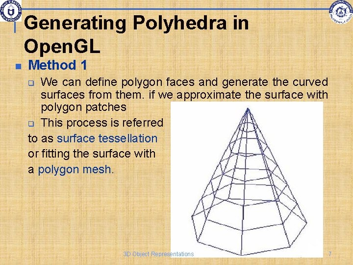
Generating Polyhedra in Open. GL Method 1 We can define polygon faces and generate the curved surfaces from them. if we approximate the surface with polygon patches q This process is referred to as surface tessellation or fitting the surface with a polygon mesh. q 3 D Object Representations 7

Generating Polyhedra in Open. GL (cont. ) In fitting polygons to a surface, we are not limited to using GL_POLYGON We can also use q q q GL_TRIANGLES GL_TRIANGLE_STRIP GL_TRIANGLE_FAN GL_QUADS GL_QUAD_STRIP 3 D Object Representations 8

Generating Polyhedra in Open. GL (cont. ) Method 2 q q Use predefined regular polyhedra from the GLUT and GLU libraries. We will look at the GLUT library functions first. 3 D Object Representations 9

The Regular Polyhedron Functions These are called the Platonic solids – all faces of the regular polyhedron are identical regular polygons. There are precisely 5 of these in 3 dimensional space 3 D Object Representations 10

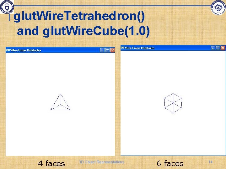
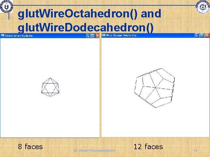
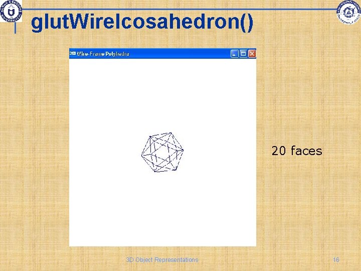
The Platonic Solids Regular tetrahedron (or triangular pyramid) has 4 faces Regular hexahedron (or cube) with 6 faces Regular octahedron with 8 faces Regular dodecahedron with 12 faces Regular icosahedron with 20 faces 3 D Object Representations 11

GLUT Library of Polyhedron Functions All are defined in model coordinates so they are specified around the origin. 5 functions produce wire frames which can be easily used Ex: glut. Wire. X(), where X is one of the names Cube, Tetrahedron, Octahedron, Dodecahedron, or Icosahedron (with the first letter capitalized). 5 functions produce polyhedra facets as shaded fill areas - the characteristics of these are determined by material and lighting properties. Ex: glut. Solid. X(), where X is as above. 3 D Object Representations 12

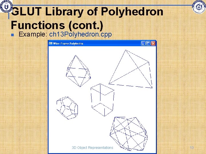
GLUT Library of Polyhedron Functions (cont. ) Example: ch 13 Polyhedron. cpp 3 D Object Representations 13

glut. Wire. Tetrahedron() and glut. Wire. Cube(1. 0) 4 faces 3 D Object Representations 6 faces 14

glut. Wire. Octahedron() and glut. Wire. Dodecahedron() 8 faces 3 D Object Representations 12 faces 15

glut. Wire. Icosahedron() 20 faces 3 D Object Representations 16

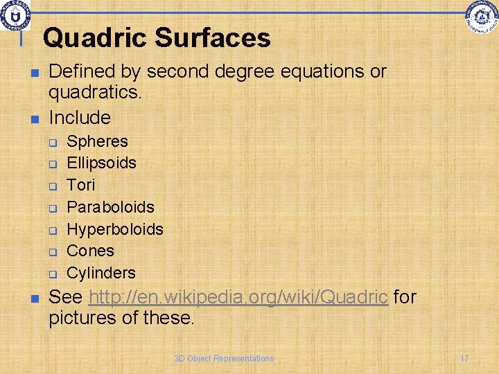
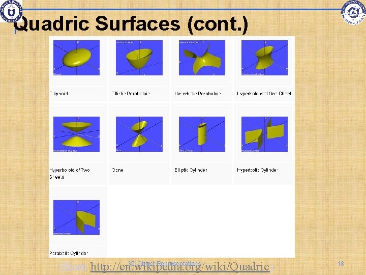
Quadric Surfaces Defined by second degree equations or quadratics. Include q q q q Spheres Ellipsoids Tori Paraboloids Hyperboloids Cones Cylinders See http: //en. wikipedia. org/wiki/Quadric for pictures of these. 3 D Object Representations 17

Quadric Surfaces (cont. ) 3 D Object Representations (from http: //en. wikipedia. org/wiki/Quadric) 18

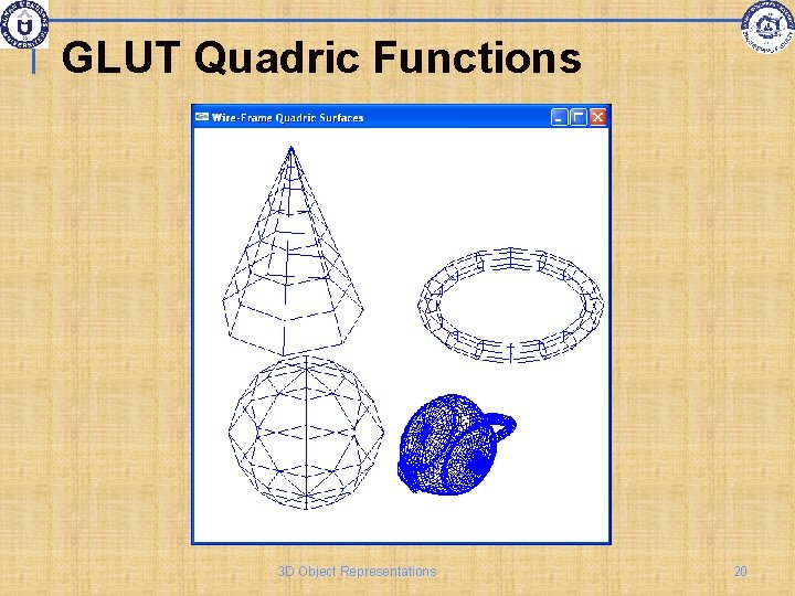
GLUT Quadric Functions – for Solids, Substitute Solid for Wire glut. Wire. Sphere(radius, slices, stacks); glut. Wire. Cone(base, height, slices, stacks); glut. Wire. Torus(inner. Radius, outer. Radius, nsides, rings); and the following is provided also! glut. Wire. Teapot(size); 3 D Object Representations 19

GLUT Quadric Functions 3 D Object Representations 20

GLU Quadric-Surface Functions GLUquadric. Obj *sphere 1; sphere 1=glu. New. Quadric( ); glu. Quadric. Draw. Style(sphere 1, GLU_LINE); glu. Sphere(sphere 1, r, n. Longitudes, n. Latitudes); 3 D Object Representations 21

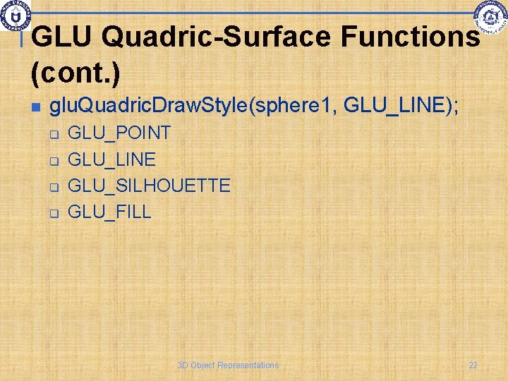
GLU Quadric-Surface Functions (cont. ) glu. Quadric. Draw. Style(sphere 1, GLU_LINE); q q GLU_POINT GLU_LINE GLU_SILHOUETTE GLU_FILL 3 D Object Representations 22

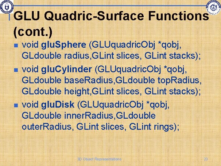
GLU Quadric-Surface Functions (cont. ) void glu. Sphere (GLUquadric. Obj *qobj, GLdouble radius, GLint slices, GLint stacks); void glu. Cylinder (GLUquadric. Obj *qobj, GLdouble base. Radius, GLdouble top. Radius, GLdouble height, GLint slices, GLint stacks); void glu. Disk (GLUquadric. Obj *qobj, GLdouble inner. Radius, GLdouble outer. Radius, GLint slices, GLint rings); 3 D Object Representations 23

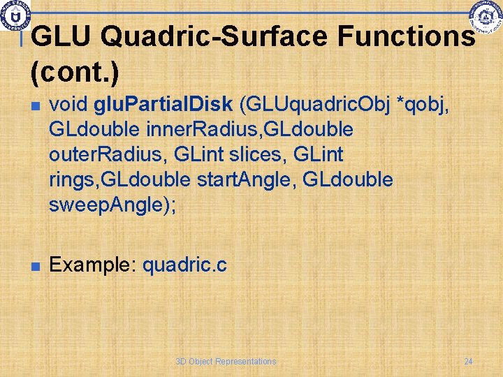
GLU Quadric-Surface Functions (cont. ) void glu. Partial. Disk (GLUquadric. Obj *qobj, GLdouble inner. Radius, GLdouble outer. Radius, GLint slices, GLint rings, GLdouble start. Angle, GLdouble sweep. Angle); Example: quadric. c 3 D Object Representations 24

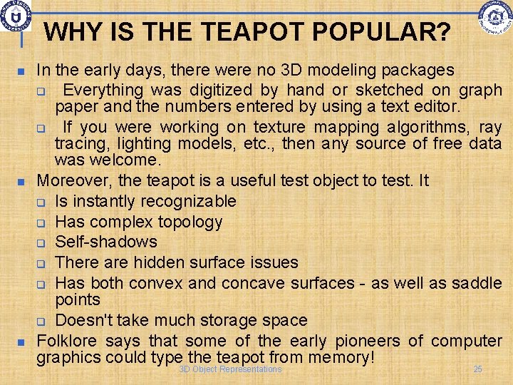
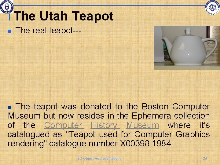
WHY IS THE TEAPOT POPULAR? In the early days, there were no 3 D modeling packages q Everything was digitized by hand or sketched on graph paper and the numbers entered by using a text editor. q If you were working on texture mapping algorithms, ray tracing, lighting models, etc. , then any source of free data was welcome. Moreover, the teapot is a useful test object to test. It q Is instantly recognizable q Has complex topology q Self-shadows q There are hidden surface issues q Has both convex and concave surfaces - as well as saddle points q Doesn't take much storage space Folklore says that some of the early pioneers of computer graphics could type the teapot from memory! 3 D Object Representations 25

The Utah Teapot The real teapot--- The teapot was donated to the Boston Computer Museum but now resides in the Ephemera collection of the Computer History Museum where it's catalogued as "Teapot used for Computer Graphics rendering" catalogue number X 00398. 1984. 3 D Object Representations 26

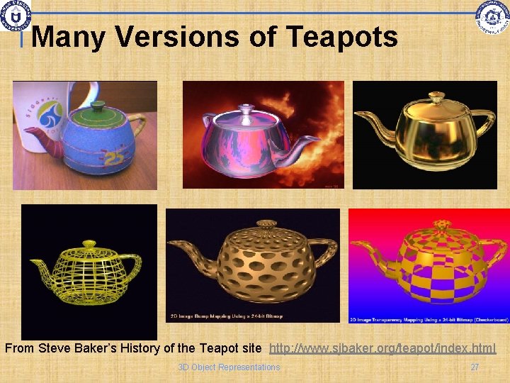
Many Versions of Teapots From Steve Baker’s History of the Teapot site: http: //www. sjbaker. org/teapot/index. html 3 D Object Representations 27

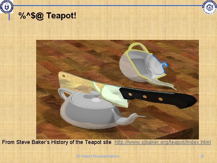
%^$@ Teapot! From Steve Baker’s History of the Teapot site: http: //www. sjbaker. org/teapot/index. html. 3 D Object Representations 28

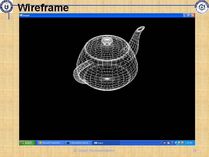
Wireframe 3 D Object Representations 29

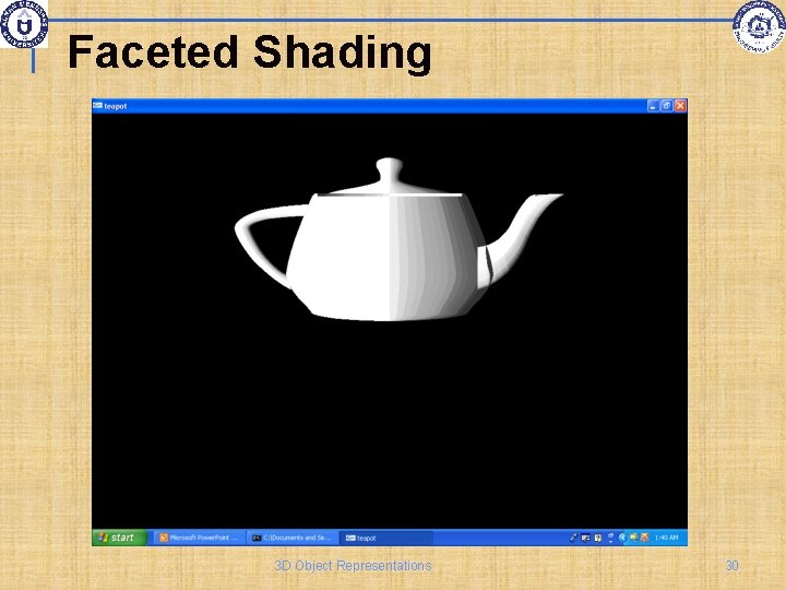
Faceted Shading 3 D Object Representations 30

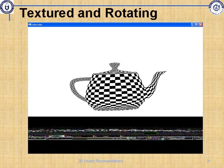
Textured and Rotating 3 D Object Representations 31

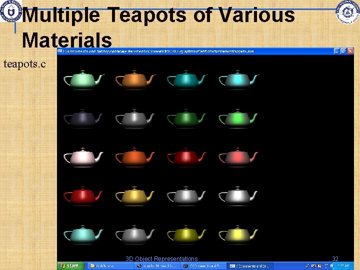
Multiple Teapots of Various Materials teapots. c 3 D Object Representations 32

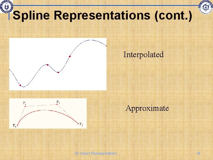
Spline Representations Splines are used to design curve and surface shapes like automobile bodies, aircraft surfaces, etc. Control points q Interpolation q Set of coordinates used to specify a curve, which indicate the general shape of the curve All the control points are connected Approximate q Some or all control points are not on the curve path 3 D Object Representations 33

Spline Representations (cont. ) Interpolated Approximate 3 D Object Representations 34

Bézier Spline Curves Developed by French engineer Pierre Bézier for use in the design of Renault automobile bodies Easy to implement q Widely used in CAD systems, graphics, drawing and painting packages 3 D Object Representations 35

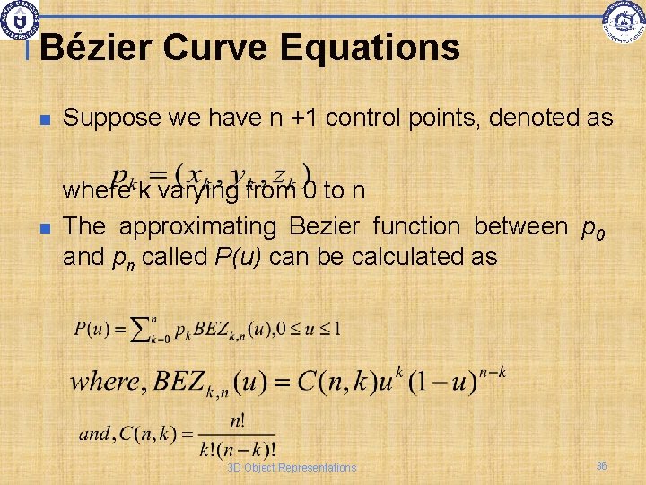
Bézier Curve Equations Suppose we have n +1 control points, denoted as where k varying from 0 to n The approximating Bezier function between p 0 and pn called P(u) can be calculated as 3 D Object Representations 36

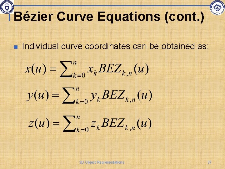
Bézier Curve Equations (cont. ) Individual curve coordinates can be obtained as: 3 D Object Representations 37

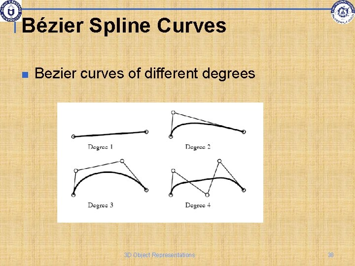
Bézier Spline Curves Bezier curves of different degrees 3 D Object Representations 38

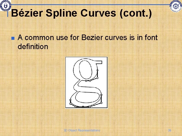
Bézier Spline Curves (cont. ) A common use for Bezier curves is in font definition 3 D Object Representations 39

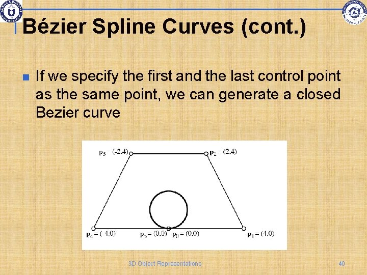
Bézier Spline Curves (cont. ) If we specify the first and the last control point as the same point, we can generate a closed Bezier curve 3 D Object Representations 40

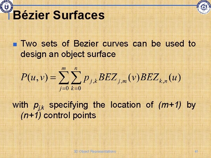
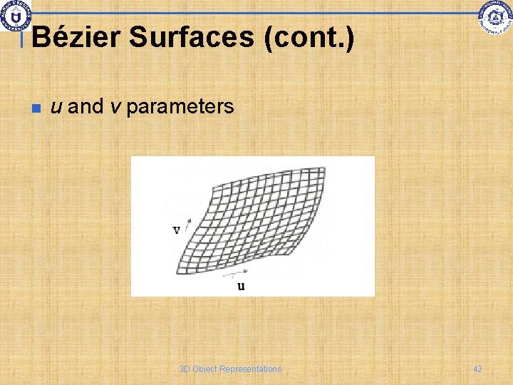
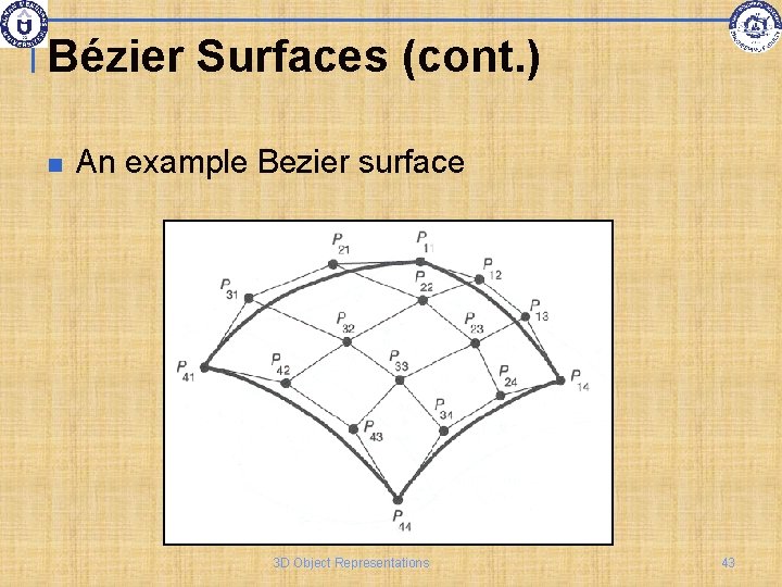
Bézier Surfaces Two sets of Bezier curves can be used to design an object surface with pj, k specifying the location of (m+1) by (n+1) control points 3 D Object Representations 41

Bézier Surfaces (cont. ) u and v parameters 3 D Object Representations 42

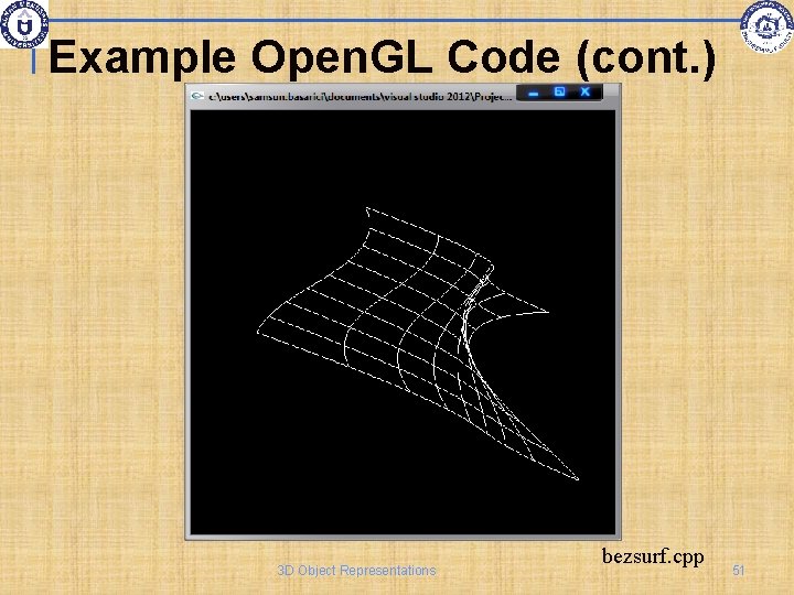
Bézier Surfaces (cont. ) An example Bezier surface 3 D Object Representations 43

Open. GL Approximation Spline Functions Bezier splines and B-splines can be displayed using Open. GL functions The core library contains Bezier functions, and GLU has B-spline functions Bezier functions are often hardware implemented 3 D Object Representations 44

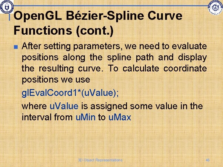
Open. GL Bézier-Spline Curve Functions We specify parameters and activate the routines for Bezier-curve display with gl. Map 1*(GL_MAP 1_VERTEX_3, u. Min, u. Max, stride, n. Pts, *ctrl. Pts); gl. Enable(GL_MAP 1_VERTEX_3); and deactivate with q q gl. Disable(GL_MAP 1_VERTEX_3); u. Min and u. Max are typically 0 and 1. 0 stride=3 for 3 D n. Pts is the number of control points ctrl. Pts is the array of control points 3 D Object Representations 45

Open. GL Bézier-Spline Curve Functions (cont. ) After setting parameters, we need to evaluate positions along the spline path and display the resulting curve. To calculate coordinate positions we use gl. Eval. Coord 1*(u. Value); where u. Value is assigned some value in the interval from u. Min to u. Max 3 D Object Representations 46

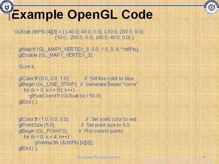
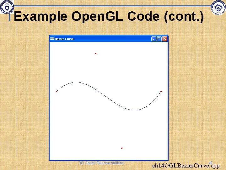
Example Open. GL Code GLfloat ctrl. Pts [4][3] = { {-40. 0, 0. 0}, {-10. 0, 200. 0, 0. 0}, {10. 0, -200. 0, 0. 0}, {40. 0, 0. 0} }; gl. Map 1 f (GL_MAP 1_VERTEX_3, 0. 0, 1. 0, 3, 4, *ctrl. Pts); gl. Enable (GL_MAP 1_VERTEX_3); GLint k; gl. Color 3 f (0. 0, 1. 0); // Set line color to blue. gl. Begin (GL_LINE_STRIP); // Generate Bezier "curve". for (k = 0; k <= 50; k++) gl. Eval. Coord 1 f (GLfloat (k) / 50. 0); gl. End ( ); gl. Color 3 f (1. 0, 0. 0); // Set point color to red. gl. Point. Size (5. 0); // Set point size to 5. 0. gl. Begin (GL_POINTS); // Plot control points. for (k = 0; k < 4; k++) gl. Vertex 3 fv (&ctrl. Pts [k][0]); gl. End ( ); 3 D Object Representations 47 prog 8 OGLBezier. Curve. cpp

Example Open. GL Code (cont. ) 3 D Object Representations 48 ch 14 OGLBezier. Curve. cpp

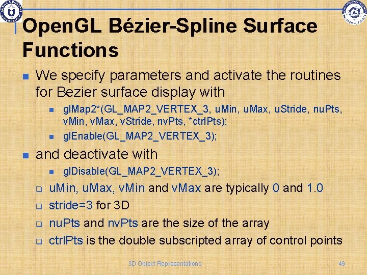
Open. GL Bézier-Spline Surface Functions We specify parameters and activate the routines for Bezier surface display with gl. Map 2*(GL_MAP 2_VERTEX_3, u. Min, u. Max, u. Stride, nu. Pts, v. Min, v. Max, v. Stride, nv. Pts, *ctrl. Pts); gl. Enable(GL_MAP 2_VERTEX_3); and deactivate with q q gl. Disable(GL_MAP 2_VERTEX_3); u. Min, u. Max, v. Min and v. Max are typically 0 and 1. 0 stride=3 for 3 D nu. Pts and nv. Pts are the size of the array ctrl. Pts is the double subscripted array of control points 3 D Object Representations 49

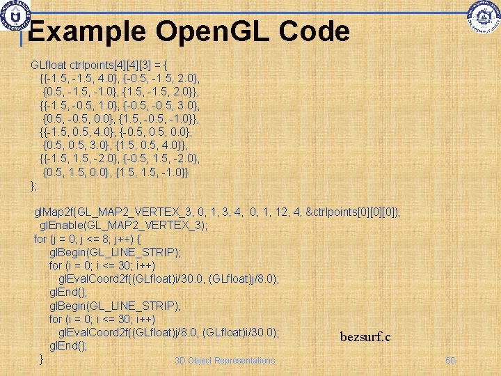
Example Open. GL Code GLfloat ctrlpoints[4][4][3] = { {{-1. 5, 4. 0}, {-0. 5, -1. 5, 2. 0}, {0. 5, -1. 0}, {1. 5, -1. 5, 2. 0}}, {{-1. 5, -0. 5, 1. 0}, {-0. 5, 3. 0}, {0. 5, -0. 5, 0. 0}, {1. 5, -0. 5, -1. 0}}, {{-1. 5, 0. 5, 4. 0}, {-0. 5, 0. 0}, {0. 5, 3. 0}, {1. 5, 0. 5, 4. 0}}, {{-1. 5, -2. 0}, {-0. 5, 1. 5, -2. 0}, {0. 5, 1. 5, 0. 0}, {1. 5, -1. 0}} }; gl. Map 2 f(GL_MAP 2_VERTEX_3, 0, 1, 3, 4, 0, 1, 12, 4, &ctrlpoints[0][0][0]); gl. Enable(GL_MAP 2_VERTEX_3); for (j = 0; j <= 8; j++) { gl. Begin(GL_LINE_STRIP); for (i = 0; i <= 30; i++) gl. Eval. Coord 2 f((GLfloat)i/30. 0, (GLfloat)j/8. 0); gl. End(); gl. Begin(GL_LINE_STRIP); for (i = 0; i <= 30; i++) gl. Eval. Coord 2 f((GLfloat)j/8. 0, (GLfloat)i/30. 0); bezsurf. c gl. End(); } 3 D Object Representations 50

Example Open. GL Code (cont. ) 3 D Object Representations bezsurf. cpp 51

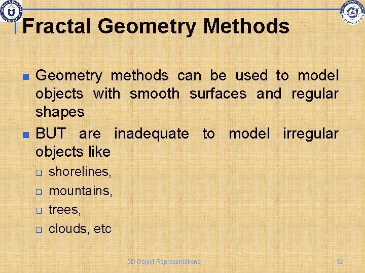
Fractal Geometry Methods Geometry methods can be used to model objects with smooth surfaces and regular shapes BUT are inadequate to model irregular objects like q q shorelines, mountains, trees, clouds, etc 3 D Object Representations 52

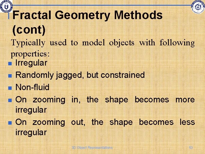
Fractal Geometry Methods (cont) Typically used to model objects with following properties: Irregular Randomly jagged, but constrained Non-fluid On zooming in, the shape becomes more irregular On zooming out, the shape becomes less irregular 3 D Object Representations 53

Fractal Geometry Methods (cont. ) A fractal object has two basic characteristics q Infinite detail at every point q If we zoom in, we see more detail of the object Self-similarity between object parts and the overall features of the object 3 D Object Representations 54

Fractal Generation Procedures A fractal object is generated by repeatedly applying a specified transformation function to points within a region of space If P 0=(x 0, y 0, z 0) then q P 1=F(P 0 ), P 2=F(P 1 ), P 3=F(P 2 ), … Transformation function can be applied to points or to a set of primitives such as lines, curves, color areas or surfaces 3 D Object Representations 55

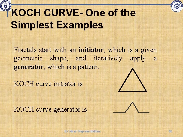
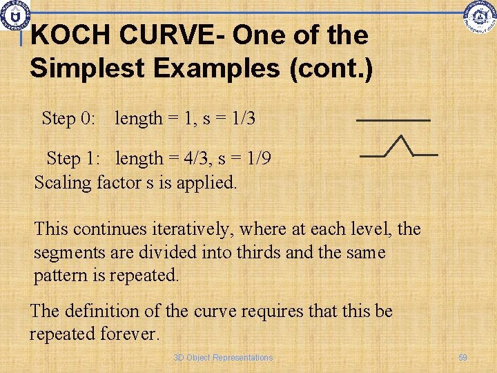
KOCH CURVE- One of the Simplest Examples Fractals start with an initiator, which is a given geometric shape, and iteratively apply a generator, which is a pattern. KOCH curve initiator is KOCH curve generator is 3 D Object Representations 56

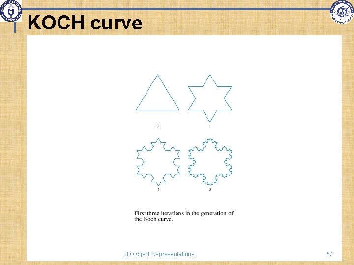
KOCH curve 3 D Object Representations 57

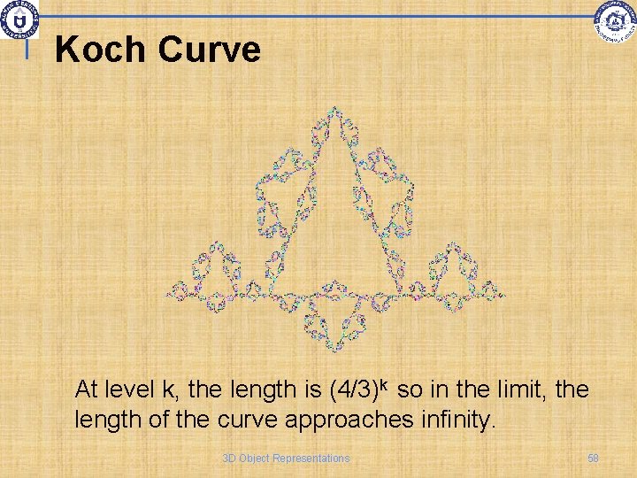
Koch Curve At level k, the length is (4/3)k so in the limit, the length of the curve approaches infinity. 3 D Object Representations 58

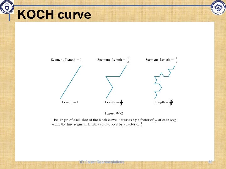
KOCH CURVE- One of the Simplest Examples (cont. ) Step 0: length = 1, s = 1/3 Step 1: length = 4/3, s = 1/9 Scaling factor s is applied. This continues iteratively, where at each level, the segments are divided into thirds and the same pattern is repeated. The definition of the curve requires that this be repeated forever. 3 D Object Representations 59

KOCH curve 3 D Object Representations 60

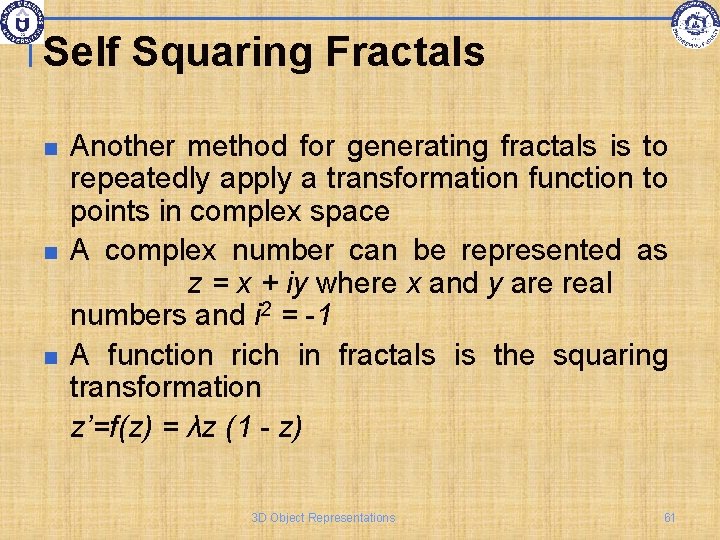
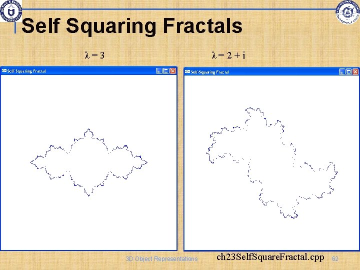
Self Squaring Fractals Another method for generating fractals is to repeatedly apply a transformation function to points in complex space A complex number can be represented as z = x + iy where x and y are real numbers and i 2 = -1 A function rich in fractals is the squaring transformation z’=f(z) = λz (1 - z) 3 D Object Representations 61

Self Squaring Fractals λ=3 λ=2+i 3 D Object Representations ch 23 Self. Square. Fractal. cpp 62

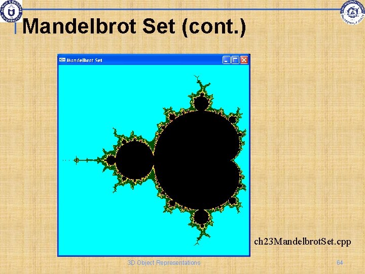
Mandelbrot Set Squaring functions were difficult to analyze without the aid of a computer Using more sophisticated computer graphics techniques, Benoit Mandelbrot studied this function and found the set of points known as Mandelbrot set 3 D Object Representations 63

Mandelbrot Set (cont. ) ch 23 Mandelbrot. Set. cpp 3 D Object Representations 64

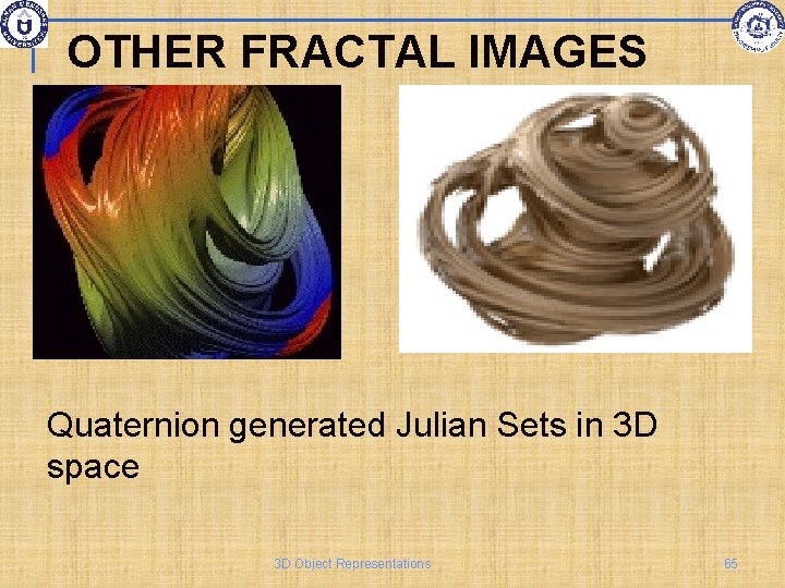
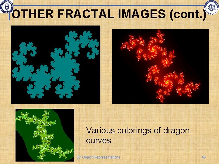
OTHER FRACTAL IMAGES Quaternion generated Julian Sets in 3 D space 3 D Object Representations 65

OTHER FRACTAL IMAGES (cont. ) Various colorings of dragon curves 3 D Object Representations 66

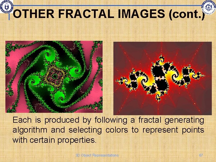
OTHER FRACTAL IMAGES (cont. ) Each is produced by following a fractal generating algorithm and selecting colors to represent points with certain properties. 3 D Object Representations 67

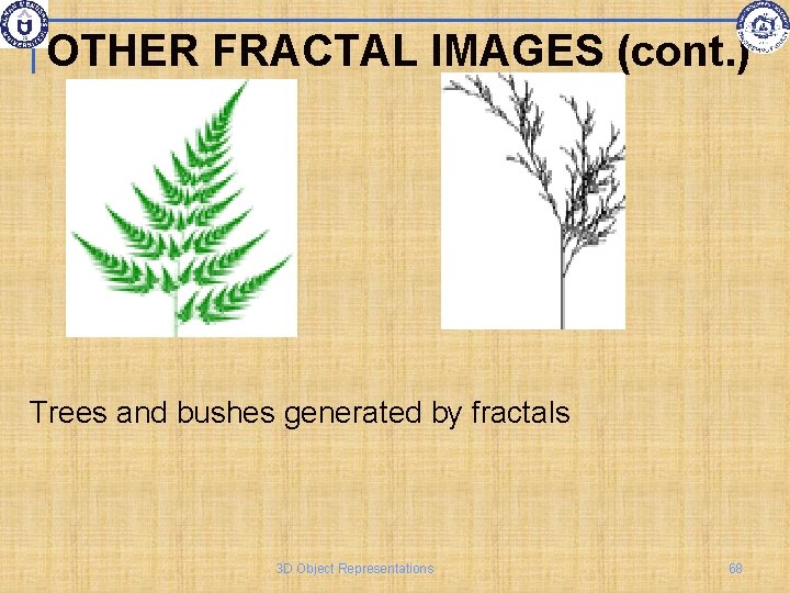
OTHER FRACTAL IMAGES (cont. ) Trees and bushes generated by fractals 3 D Object Representations 68

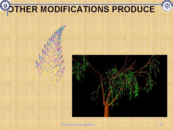
OTHER MODIFICATIONS PRODUCE 3 D Object Representations 69

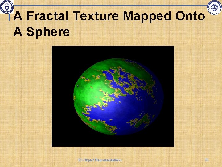
A Fractal Texture Mapped Onto A Sphere 3 D Object Representations 70

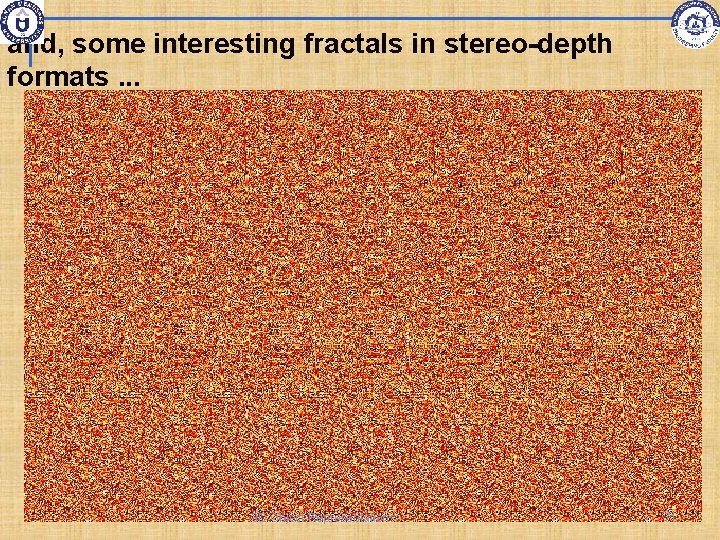
and, some interesting fractals in stereo-depth formats. . . 3 D Object Representations 71

3 D Object Representations 72

3 D Object Representations 73

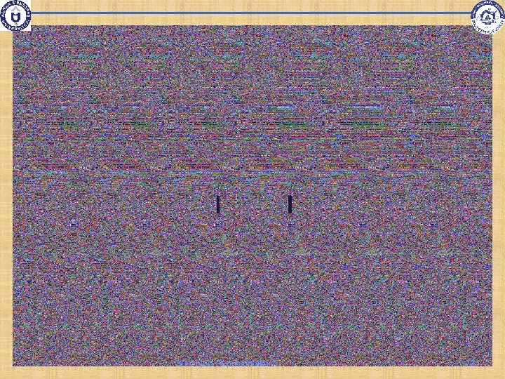
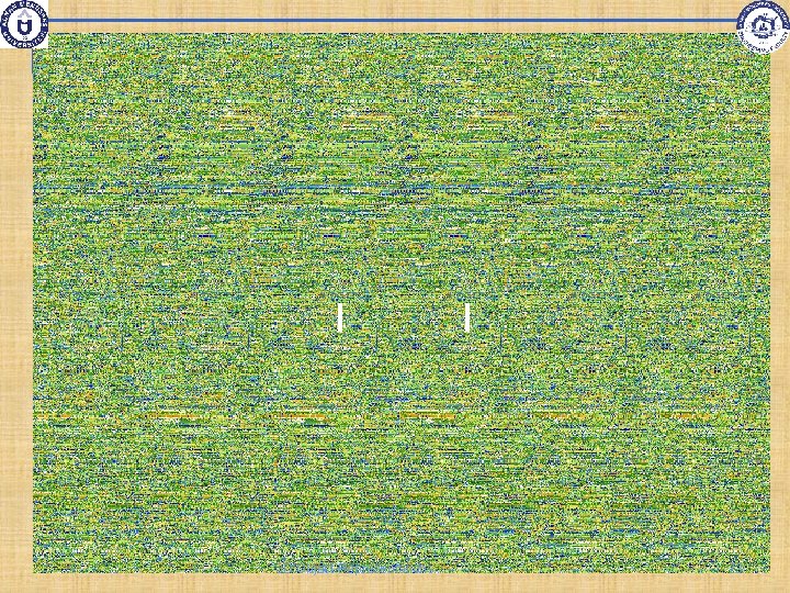
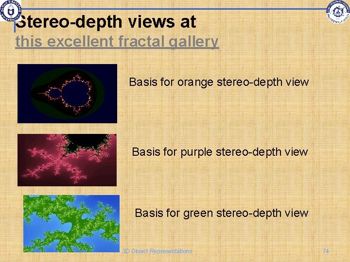
Stereo-depth views at this excellent fractal gallery Basis for orange stereo-depth view Basis for purple stereo-depth view Basis for green stereo-depth view 3 D Object Representations 74

References Donald Hearn, M. Pauline Baker, Warren R. Carithers, “Computer Graphics with Open. GL, 4 th Edition”; Pearson, 2011 Sumanta Guha, “Computer Graphics Through Open. GL: From Theory to Experiments”, CRC Press, 2010 Edward Angel, “Interactive Computer Graphics. A Top-Down Approach Using Open. GL”, Addison. Wesley, 2005 75