Analysis Design of Algorithms CSCE 321 Prof Amr

Analysis & Design of Algorithms (CSCE 321) Prof. Amr Goneid Department of Computer Science, AUC Part 8. Greedy Algorithms Prof. Amr Goneid, AUC 1

Greedy Algorithms Prof. Amr Goneid, AUC 2

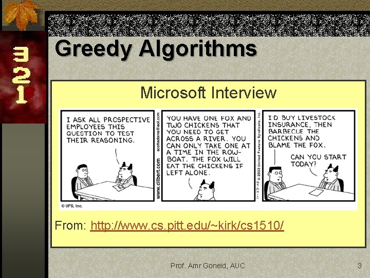
Greedy Algorithms Microsoft Interview From: http: //www. cs. pitt. edu/~kirk/cs 1510/ Prof. Amr Goneid, AUC 3

Greedy Algorithms n The General Method n Continuous Knapsack Problem n Optimal Merge Patterns Prof. Amr Goneid, AUC 4

1. Greedy Algorithms Methodology: n Start with a solution to a small subproblem n Build up to the whole problem n Make choices that look good in the short term but not necessarily in the long term Prof. Amr Goneid, AUC 5

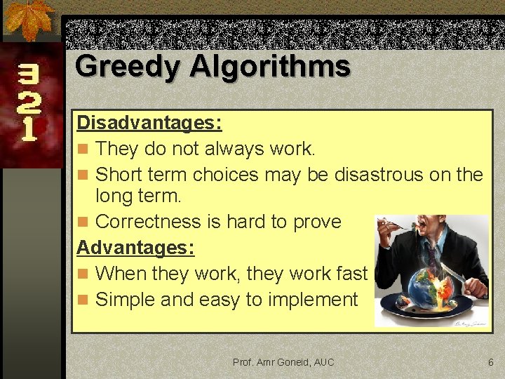
Greedy Algorithms Disadvantages: n They do not always work. n Short term choices may be disastrous on the long term. n Correctness is hard to prove Advantages: n When they work, they work fast n Simple and easy to implement Prof. Amr Goneid, AUC 6

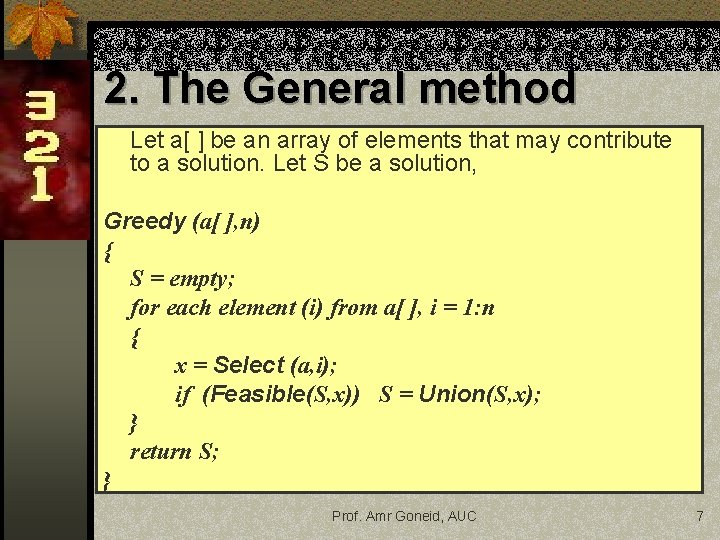
2. The General method Let a[ ] be an array of elements that may contribute to a solution. Let S be a solution, Greedy (a[ ], n) { S = empty; for each element (i) from a[ ], i = 1: n { x = Select (a, i); if (Feasible(S, x)) S = Union(S, x); } return S; } Prof. Amr Goneid, AUC 7

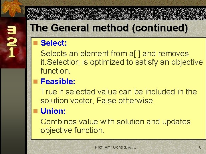
The General method (continued) n Select: Selects an element from a[ ] and removes it. Selection is optimized to satisfy an objective function. n Feasible: True if selected value can be included in the solution vector, False otherwise. n Union: Combines value with solution and updates objective function. Prof. Amr Goneid, AUC 8

3. Continuous Knapsack Problem Prof. Amr Goneid, AUC 9

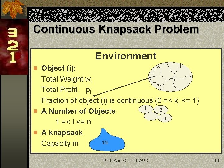
Continuous Knapsack Problem Environment n Object (i): Total Weight wi Total Profit pi Fraction of object (i) is continuous (0 =< xi <= 1) 1 2 n A Number of Objects n 1 =< i <= n n A knapsack m Capacity m Prof. Amr Goneid, AUC 10

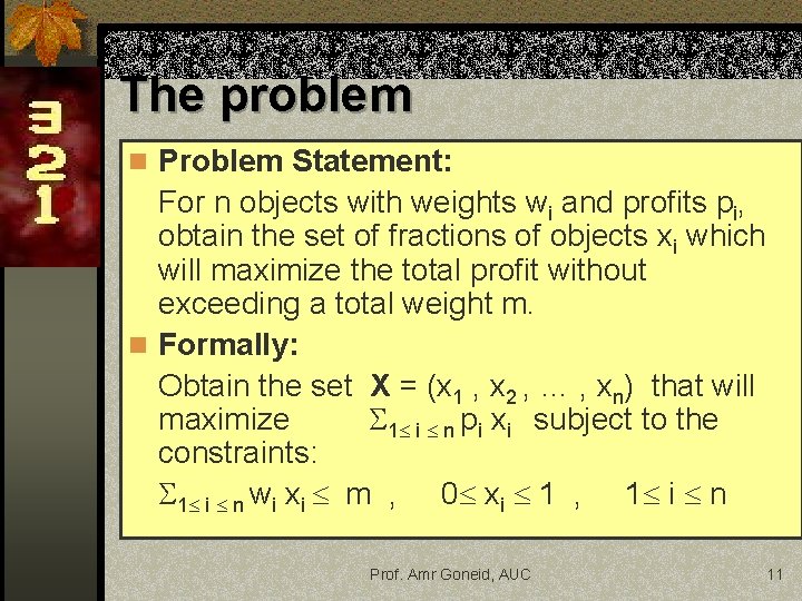
The problem n Problem Statement: For n objects with weights wi and profits pi, obtain the set of fractions of objects xi which will maximize the total profit without exceeding a total weight m. n Formally: Obtain the set X = (x 1 , x 2 , … , xn) that will maximize 1 i n pi xi subject to the constraints: 1 i n wi xi m , 0 xi 1 , 1 i n Prof. Amr Goneid, AUC 11

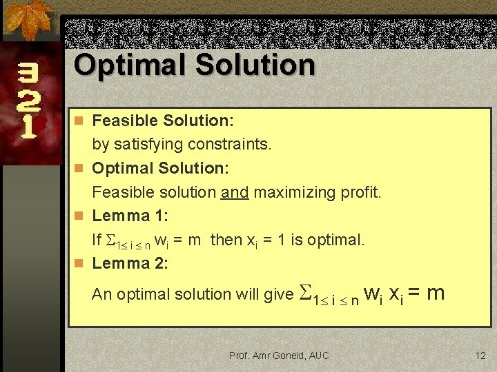
Optimal Solution n Feasible Solution: by satisfying constraints. n Optimal Solution: Feasible solution and maximizing profit. n Lemma 1: If 1 i n wi = m then xi = 1 is optimal. n Lemma 2: An optimal solution will give 1 i n wi Prof. Amr Goneid, AUC xi = m 12

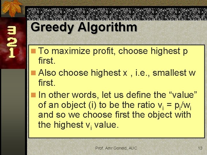
Greedy Algorithm n To maximize profit, choose highest p first. n Also choose highest x , i. e. , smallest w first. n In other words, let us define the “value” of an object (i) to be the ratio vi = pi/wi and so we choose first the object with the highest vi value. Prof. Amr Goneid, AUC 13

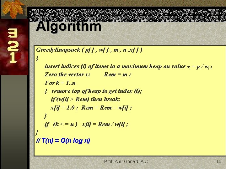
Algorithm Greedy. Knapsack ( p[ ] , w[ ] , m , n , x[ ] ) { insert indices (i) of items in a maximum heap on value vi = pi / wi ; Zero the vector x; Rem = m ; For k = 1. . n { remove top of heap to get index (i); if (w[i] > Rem) then break; x[i] = 1. 0 ; Rem = Rem – w[i] ; } if (k < = n ) x[i] = Rem / w[i] ; } // T(n) = O(n log n) Prof. Amr Goneid, AUC 14

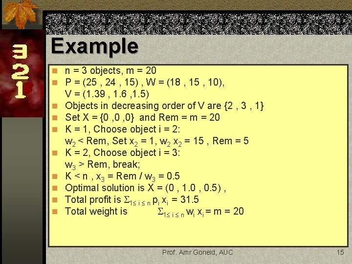
Example n n = 3 objects, m = 20 n P = (25 , 24 , 15) , W = (18 , 15 , 10), n n n n V = (1. 39 , 1. 6 , 1. 5) Objects in decreasing order of V are {2 , 3 , 1} Set X = {0 , 0} and Rem = 20 K = 1, Choose object i = 2: w 2 < Rem, Set x 2 = 1, w 2 x 2 = 15 , Rem = 5 K = 2, Choose object i = 3: w 3 > Rem, break; K < n , x 3 = Rem / w 3 = 0. 5 Optimal solution is X = (0 , 1. 0 , 0. 5) , Total profit is 1 i n pi xi = 31. 5 Total weight is 1 i n wi xi = m = 20 Prof. Amr Goneid, AUC 15

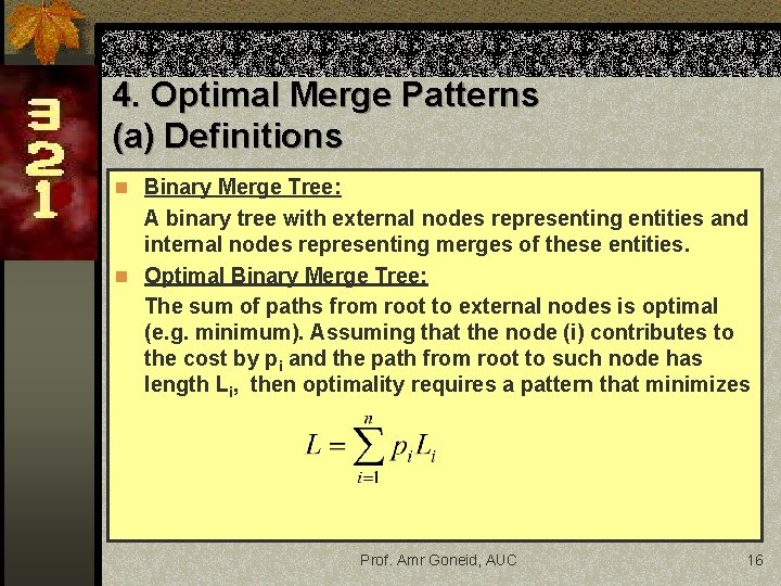
4. Optimal Merge Patterns (a) Definitions n Binary Merge Tree: A binary tree with external nodes representing entities and internal nodes representing merges of these entities. n Optimal Binary Merge Tree: The sum of paths from root to external nodes is optimal (e. g. minimum). Assuming that the node (i) contributes to the cost by pi and the path from root to such node has length Li, then optimality requires a pattern that minimizes Prof. Amr Goneid, AUC 16

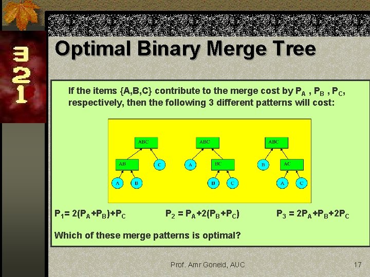
Optimal Binary Merge Tree If the items {A, B, C} contribute to the merge cost by PA , PB , PC, respectively, then the following 3 different patterns will cost: P 1= 2(PA+PB)+PC P 2 = PA+2(PB+PC) P 3 = 2 PA+PB+2 PC Which of these merge patterns is optimal? Prof. Amr Goneid, AUC 17

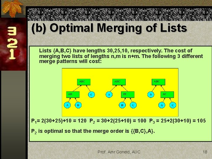
(b) Optimal Merging of Lists {A, B, C} have lengths 30, 25, 10, respectively. The cost of merging two lists of lengths n, m is n+m. The following 3 different merge patterns will cost: P 1= 2(30+25)+10 = 120 P 2 = 30+2(25+10) = 100 P 3 = 25+2(30+10) = 105 P 2 is optimal so that the merge order is {{B, C}, A}. Prof. Amr Goneid, AUC 18

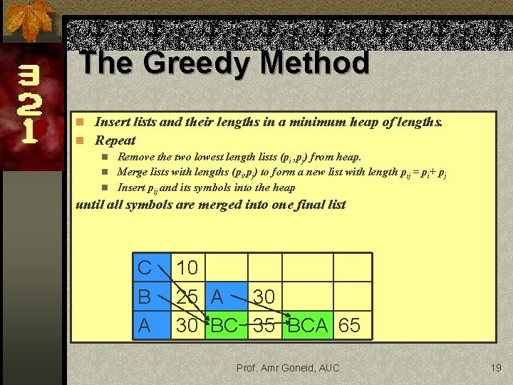
The Greedy Method n Insert lists and their lengths in a minimum heap of lengths. n Repeat Remove the two lowest length lists (pi , pj) from heap. n Merge lists with lengths (pi, pj) to form a new list with length pij = pi+ pj n Insert pij and its symbols into the heap n until all symbols are merged into one final list C B A 10 25 A 30 30 BC 35 BCA 65 Prof. Amr Goneid, AUC 19

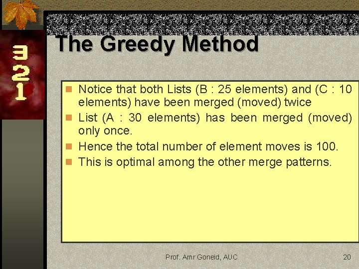
The Greedy Method n Notice that both Lists (B : 25 elements) and (C : 10 elements) have been merged (moved) twice n List (A : 30 elements) has been merged (moved) only once. n Hence the total number of element moves is 100. n This is optimal among the other merge patterns. Prof. Amr Goneid, AUC 20

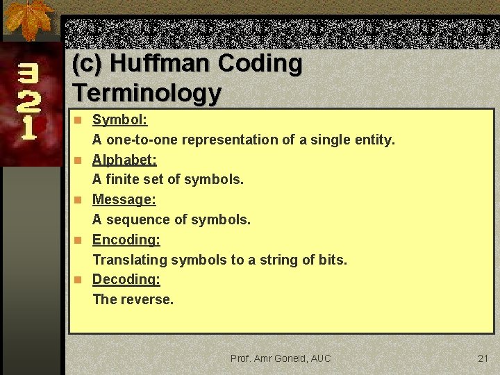
(c) Huffman Coding Terminology n Symbol: n n A one-to-one representation of a single entity. Alphabet: A finite set of symbols. Message: A sequence of symbols. Encoding: Translating symbols to a string of bits. Decoding: The reverse. Prof. Amr Goneid, AUC 21

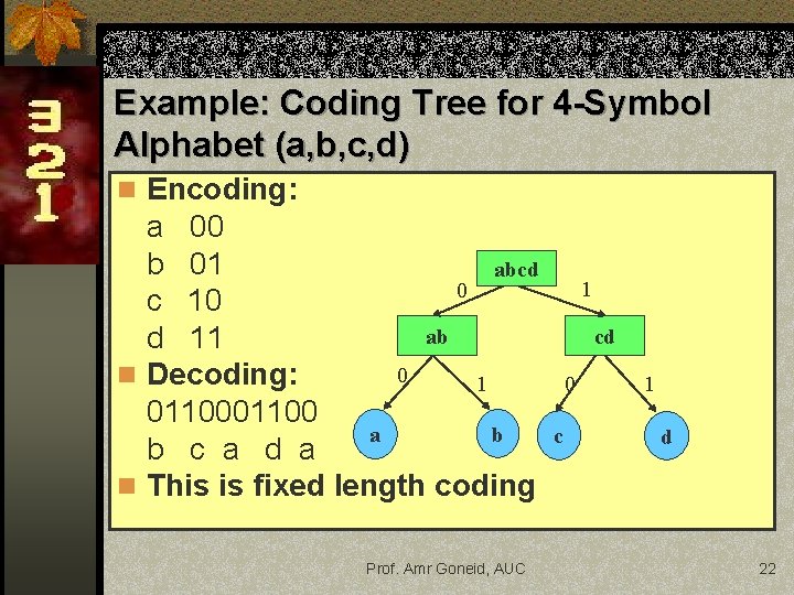
Example: Coding Tree for 4 -Symbol Alphabet (a, b, c, d) n Encoding: a 00 b 01 abcd 0 c 10 ab d 11 0 n Decoding: 1 01100 b a b c a d a n This is fixed length coding Prof. Amr Goneid, AUC 1 cd 0 c 1 d 22

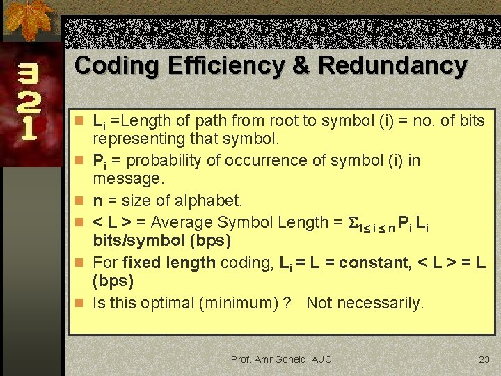
Coding Efficiency & Redundancy n Li =Length of path from root to symbol (i) = no. of bits n n n representing that symbol. Pi = probability of occurrence of symbol (i) in message. n = size of alphabet. < L > = Average Symbol Length = 1 i n Pi Li bits/symbol (bps) For fixed length coding, Li = L = constant, < L > = L (bps) Is this optimal (minimum) ? Not necessarily. Prof. Amr Goneid, AUC 23

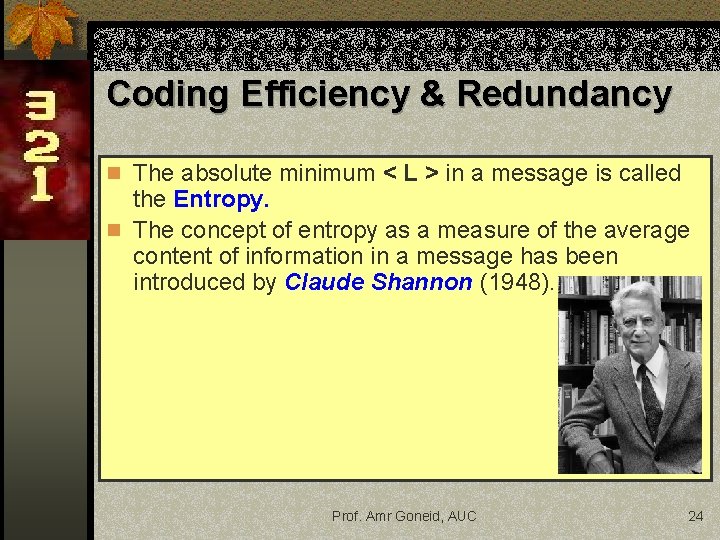
Coding Efficiency & Redundancy n The absolute minimum < L > in a message is called the Entropy. n The concept of entropy as a measure of the average content of information in a message has been introduced by Claude Shannon (1948). Prof. Amr Goneid, AUC 24

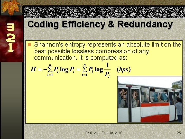
Coding Efficiency & Redundancy n Shannon's entropy represents an absolute limit on the best possible lossless compression of any communication. It is computed as: Prof. Amr Goneid, AUC 25

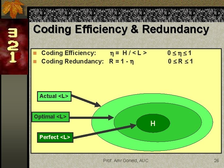
Coding Efficiency & Redundancy = H/<L> n Coding Redundancy: R = 1 - 0 1 0 R 1 n Coding Efficiency: Actual <L> Optimal <L> H Perfect <L> Prof. Amr Goneid, AUC 26

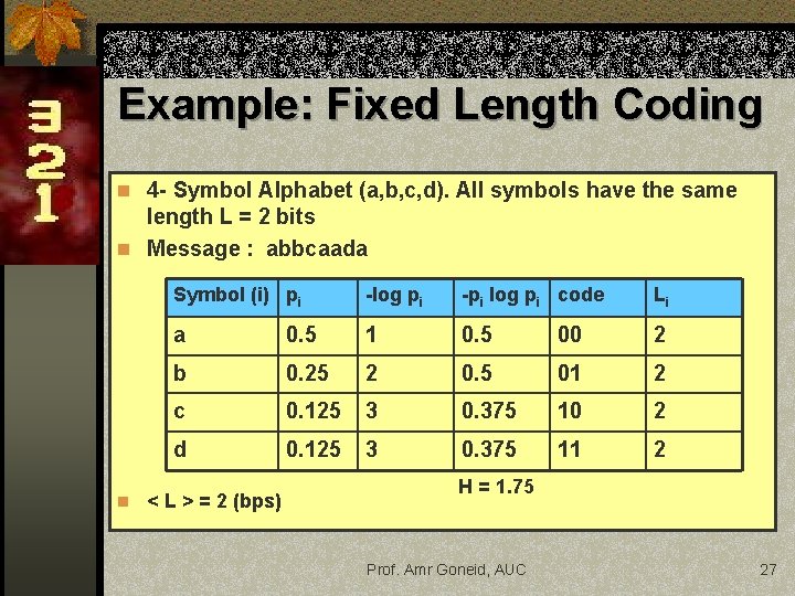
Example: Fixed Length Coding n 4 - Symbol Alphabet (a, b, c, d). All symbols have the same length L = 2 bits n Message : abbcaada Symbol (i) pi -log pi -pi log pi code Li a 0. 5 1 0. 5 00 2 b 0. 25 2 0. 5 01 2 c 0. 125 3 0. 375 10 2 d 0. 125 3 0. 375 11 2 n < L > = 2 (bps) H = 1. 75 Prof. Amr Goneid, AUC 27

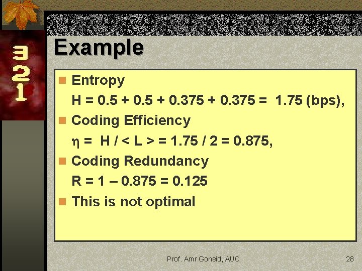
Example n Entropy H = 0. 5 + 0. 375 = 1. 75 (bps), n Coding Efficiency = H / < L > = 1. 75 / 2 = 0. 875, n Coding Redundancy R = 1 – 0. 875 = 0. 125 n This is not optimal Prof. Amr Goneid, AUC 28

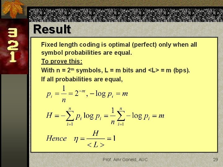
Result Fixed length coding is optimal (perfect) only when all symbol probabilities are equal. To prove this: With n = 2 m symbols, L = m bits and <L> = m (bps). If all probabilities are equal, Prof. Amr Goneid, AUC 29

Variable Length Coding (Huffman Coding) The problem: n Given a set of symbols and their probabilities n Find a set of binary codewords that minimize the average length of the symbols Prof. Amr Goneid, AUC 30

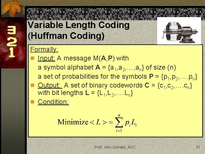
Variable Length Coding (Huffman Coding) Formally: n Input: A message M(A, P) with a symbol alphabet A = {a 1, a 2, …, an} of size (n) a set of probabilities for the symbols P = {p 1, p 2, …. pn} n Output: A set of binary codewords C = {c 1, c 2, …. cn} with bit lengths L = {L 1, L 2, …. Ln} n Condition: Prof. Amr Goneid, AUC 31

Variable Length Coding (Huffman Coding) n To achieve optimality, we use optimal binary merge trees to code symbols of unequal probabilities. n Huffman Coding: More frequent symbols occur nearer to the root ( shorter code lengths), less frequent symbols occur at deeper levels (longer code lengths). Prof. Amr Goneid, AUC 32

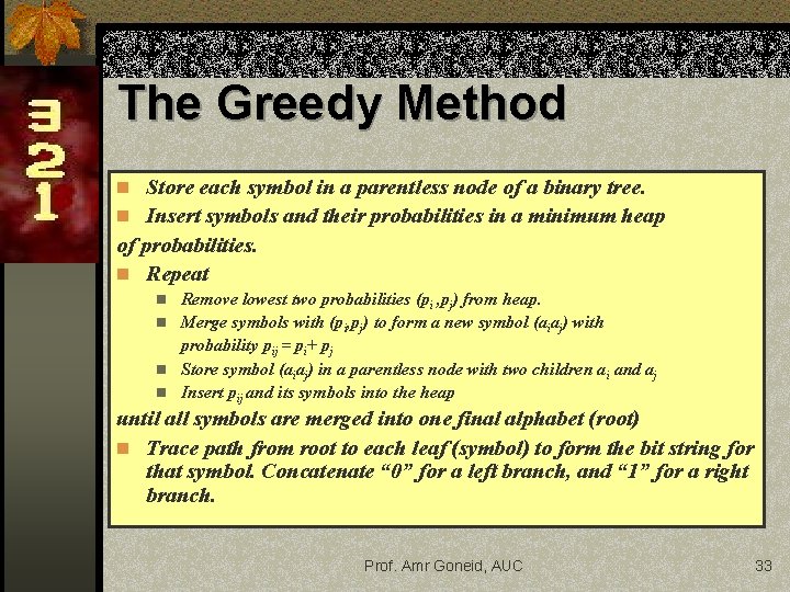
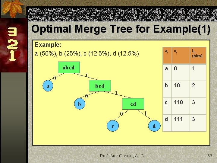
The Greedy Method n Store each symbol in a parentless node of a binary tree. n Insert symbols and their probabilities in a minimum heap of probabilities. n Repeat Remove lowest two probabilities (pi , pj) from heap. n Merge symbols with (pi, pj) to form a new symbol (aiaj) with probability pij = pi+ pj n Store symbol (aiaj) in a parentless node with two children ai and aj n Insert pij and its symbols into the heap n until all symbols are merged into one final alphabet (root) n Trace path from root to each leaf (symbol) to form the bit string for that symbol. Concatenate “ 0” for a left branch, and “ 1” for a right branch. Prof. Amr Goneid, AUC 33

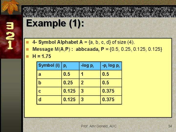
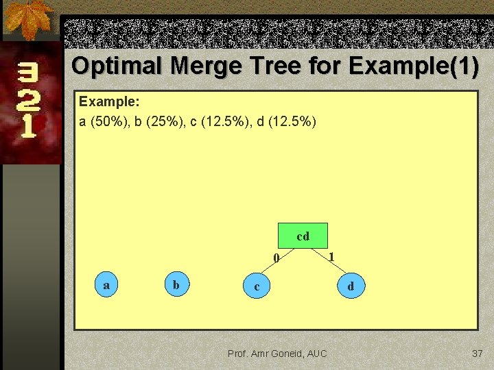
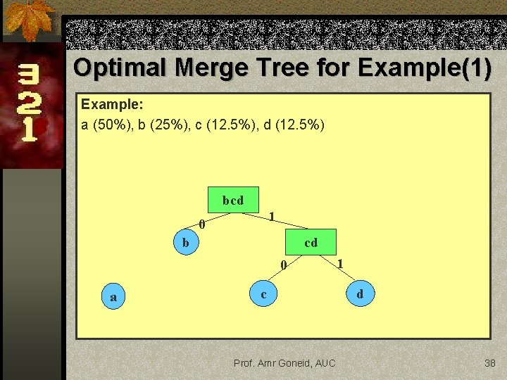
Example (1): n 4 - Symbol Alphabet A = {a, b, c, d} of size (4). n Message M(A, P) : abbcaada, P = {0. 5, 0. 25, 0. 125} n H = 1. 75 Symbol (i) pi -log pi -pi log pi a 0. 5 1 0. 5 b 0. 25 2 0. 5 c 0. 125 3 0. 375 d 0. 125 3 0. 375 Prof. Amr Goneid, AUC 34

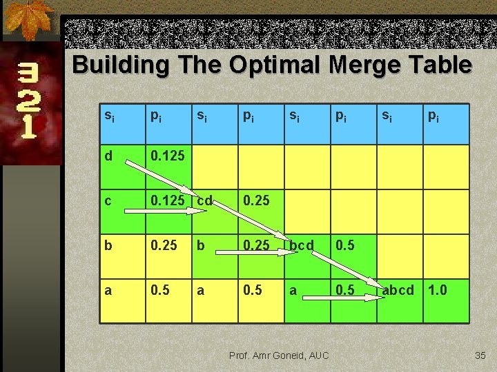
Building The Optimal Merge Table si pi d 0. 125 cd 0. 25 bcd 0. 5 a 0. 5 Prof. Amr Goneid, AUC si pi abcd 1. 0 35

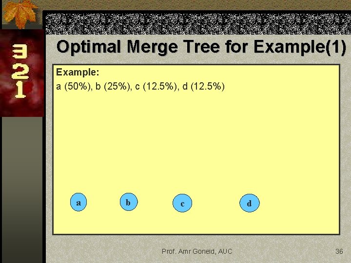
Optimal Merge Tree for Example(1) Example: a (50%), b (25%), c (12. 5%), d (12. 5%) a b c Prof. Amr Goneid, AUC d 36

Optimal Merge Tree for Example(1) Example: a (50%), b (25%), c (12. 5%), d (12. 5%) cd 0 a b c Prof. Amr Goneid, AUC 1 d 37

Optimal Merge Tree for Example(1) Example: a (50%), b (25%), c (12. 5%), d (12. 5%) bcd 1 0 cd b 0 a c Prof. Amr Goneid, AUC 1 d 38

Optimal Merge Tree for Example(1) Example: a (50%), b (25%), c (12. 5%), d (12. 5%) abcd ai ci Li (bits) a 0 1 b 10 2 c 110 3 d 111 3 1 0 bcd a 1 0 cd b 0 c Prof. Amr Goneid, AUC 1 d 39

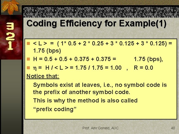
Coding Efficiency for Example(1) n < L > = ( 1* 0. 5 + 2 * 0. 25 + 3 * 0. 125) = 1. 75 (bps) n H = 0. 5 + 0. 375 = 1. 75 (bps), n = H / < L > = 1. 75 / 1. 75 = 1. 00 , R = 0. 0 Notice that: Symbols exist at leaves, i. e. , no symbol code is the prefix of another symbol code. This is why the method is also called “prefix coding” Prof. Amr Goneid, AUC 40

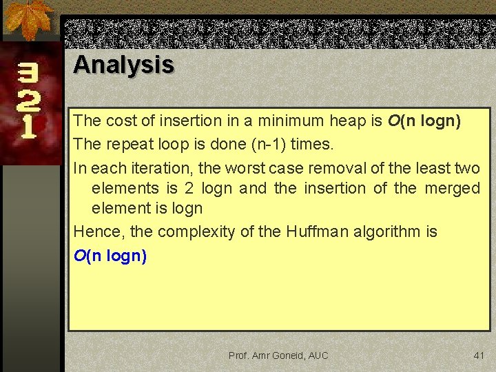
Analysis The cost of insertion in a minimum heap is O(n logn) The repeat loop is done (n-1) times. In each iteration, the worst case removal of the least two elements is 2 logn and the insertion of the merged element is logn Hence, the complexity of the Huffman algorithm is O(n logn) Prof. Amr Goneid, AUC 41

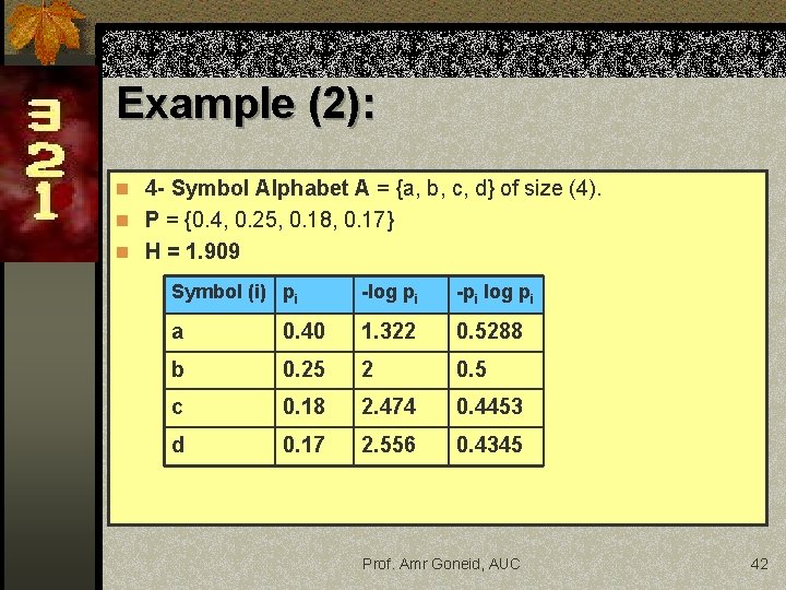
Example (2): n 4 - Symbol Alphabet A = {a, b, c, d} of size (4). n P = {0. 4, 0. 25, 0. 18, 0. 17} n H = 1. 909 Symbol (i) pi -log pi -pi log pi a 0. 40 1. 322 0. 5288 b 0. 25 2 0. 5 c 0. 18 2. 474 0. 4453 d 0. 17 2. 556 0. 4345 Prof. Amr Goneid, AUC 42

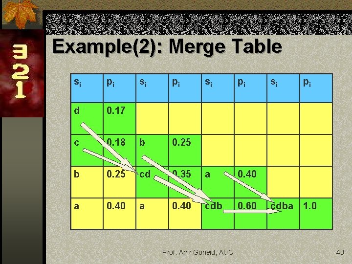
Example(2): Merge Table si pi d 0. 17 c si pi 0. 18 b 0. 25 cd 0. 35 a 0. 40 cdb 0. 60 Prof. Amr Goneid, AUC si pi cdba 1. 0 43

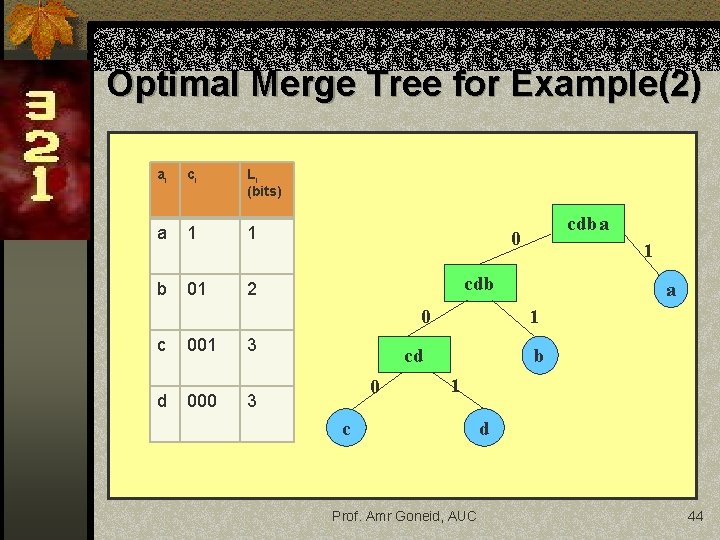
Optimal Merge Tree for Example(2) ai ci Li (bits) a 1 1 b 01 2 0 d 001 000 1 cdb 0 c cdba 3 1 cd 0 3 a b 1 c Prof. Amr Goneid, AUC d 44

Coding Efficiency for Example(2) a (40%), b (25%), c (18%), d (17%) <L> = 1. 95 bps (Optimal) H = 1. 909 = 97. 9 % R = 2. 1 % Coding is optimal (97. 9%) but not perfect Important Result: Perfect coding ( = 100 %) can be achieved only for probability values of the form 2 - m (1/2, ¼, 1/8, …etc ) Prof. Amr Goneid, AUC 45

File Compression n Variable Length Codes can be used to compress files. Symbols are initially coded using ASCII (8 -bit) fixed length codes. n Steps: 1. Determine Probabilities of symbols in file. 2. Build Merge Tree (or Table) 3. Assign variable length codes to symbols. 4. Encode symbols using new codes. 5. Save coded symbols in another file together with the symbol code table. n The Compression Ratio = < L > / 8 Prof. Amr Goneid, AUC 46

Huffman Coding Animations For examples of animations of Huffman coding, see: n http: //www. cs. pitt. edu/~kirk/cs 1501/animations Huffman. html n http: //peter. bittner. it/tugraz/huffmancoding. html Prof. Amr Goneid, AUC 47