CS 548 Spring 2016 Model and Regression Trees

CS 548 Spring 2016 Model and Regression Trees Showcase by Yanran Ma, Thanaporn Patikorn, Boya Zhou Showcasing work by Gabriele Fanelli, Juergen Gall, and Luc Van Gool on Real Time Head Pose Estimation with Random Regression Forests

References [1] Fanelli, G. ; Gall, J. ; Van Gool, L. , "Real time head pose estimation with random regression forests, " in IEEE Conference on Computer Vision and Pattern Recognition (CVPR), 2011, vol. , no. , pp. 617 -624, 20 -25 June 2011. doi: 10. 1109/CVPR. 2011. 5995458 URL: http: //ieeexplore. ieee. org/stamp. jsp? tp=&arnumber=5995458&isn umber=5995307 [2] Hastie, Trevor; Tibshirani, Robert; Friedman, Jerome (2008). The Elements of Statistical Learning (2 nd ed. ). Springer. ISBN 0 -387 -95284 -5. Page 587 -588

Outline • Application: Real Time Head Pose Estimation with Random Regression Forests • Background & Importance • Formulate the Problem – Input & Labels – Training Set & Test Set • Algorithm: Random Regression Forest • Results

Short Description This paper introduces a system that can detect head pose in real-time. The detection algorithm uses random regression forests, which utilize several regression trees to make predictions. Since images do not have typical features for tree construction, the trees were trained from sets of randomly generated rules that maximize information gain.

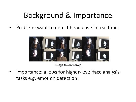
Background & Importance • Problem: want to detect head pose in real time Image taken from [1] • Importance: allows for higher-level face analysis tasks e. g. emotion detection

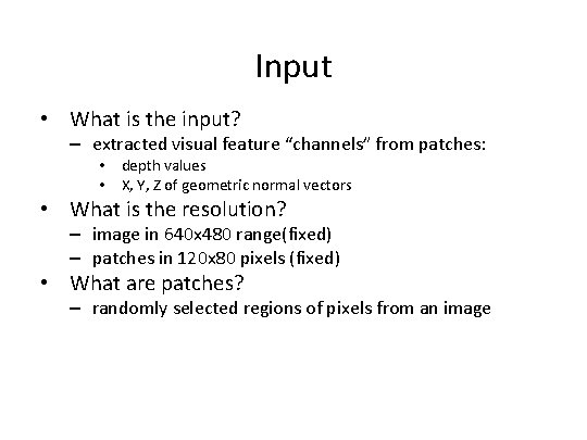
Input • What is the input? – extracted visual feature “channels” from patches: • depth values • X, Y, Z of geometric normal vectors • What is the resolution? – image in 640 x 480 range(fixed) – patches in 120 x 80 pixels (fixed) • What are patches? – randomly selected regions of pixels from an image

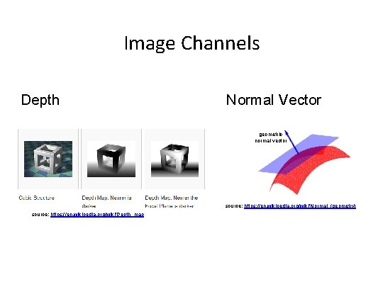
Image Channels Depth Normal Vector geometric normal vector source: https: //en. wikipedia. org/wiki/Normal_(geometry) source: https: //en. wikipedia. org/wiki/Depth_map

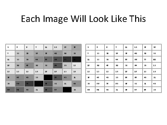
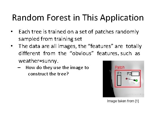
Each Image Will Look Like This 3 5 9 7 11 13 25 35 7 22 30 35 35 40 30 32 11 22 33 44 55 66 77 88 15 30 45 30 32 64 23 12 12 13 15 15 12 13 35 45 43 23 95 65 43 21 23 56 75 93 65 32 21 43 56 58 43 21 65 47 95 23

Input • What is the input? – extracted visual feature “channels” from patches: • depth values • X, Y, Z of geometric normal vectors • What is the resolution? – image in 640 x 480 range(fixed) – patches in 120 x 80 pixels (fixed) • What are patches? – randomly selected regions of pixels from an image

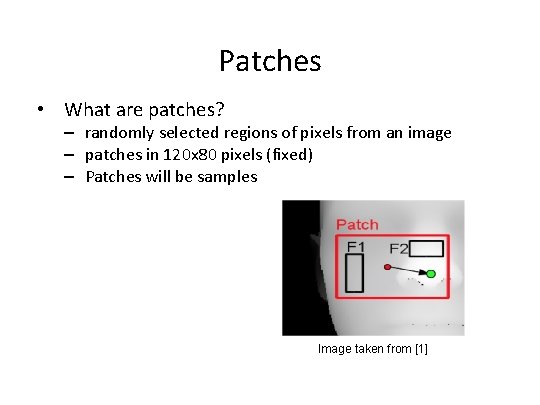
Patches • What are patches? – randomly selected regions of pixels from an image – patches in 120 x 80 pixels (fixed) – Patches will be samples Image taken from [1]

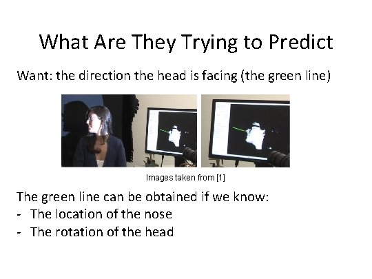
What Are They Trying to Predict Want: the direction the head is facing (the green line) Images taken from [1] The green line can be obtained if we know: - The location of the nose - The rotation of the head

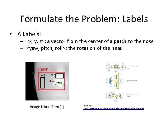
Formulate the Problem: Labels • 6 Labels: – <x, y, z>: a vector from the center of a patch to the nose – <yaw, pitch, roll>: the rotation of the head Image taken from [1] Source: http: //howthingsfly. si. edu/flight-dynamics/roll-pitch-and-yaw

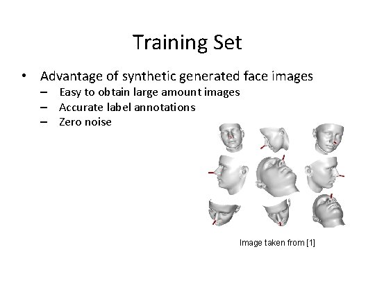
Training Set • Advantage of synthetic generated face images – Easy to obtain large amount images – Accurate label annotations – Zero noise Image taken from [1]

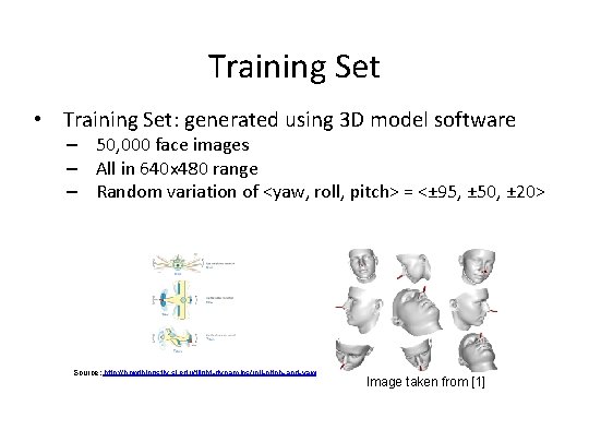
Training Set • Training Set: generated using 3 D model software – 50, 000 face images – All in 640 x 480 range – Random variation of <yaw, roll, pitch> = <± 95, ± 50, ± 20> Source: http: //howthingsfly. si. edu/flight-dynamics/roll-pitch-and-yaw Image taken from [1]

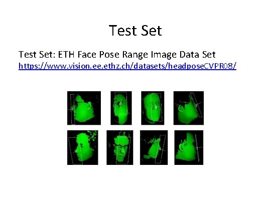
Test Set: ETH Face Pose Range Image Data Set https: //www. vision. ee. ethz. ch/datasets/headpose. CVPR 08/

Test Set • Test Set: ETH Face Pose Range Image Data Set – Well-known published head pose data set – Big data set: over 10, 000 images – Realistic data – Ground truth (labels) is provided – Each image is 640 x 480 – head pose range: ± 90 yaw and ± 45 pitch https: //www. vision. ee. ethz. ch/datasets/headpose. CVPR 08/

What is Random Regression Forest? • • A forest is a group of trees Random: each tree is trained with only a random subset of training set – Random subset of features – Random subsamples • Each tree behaves just like regular decision/regression tree.

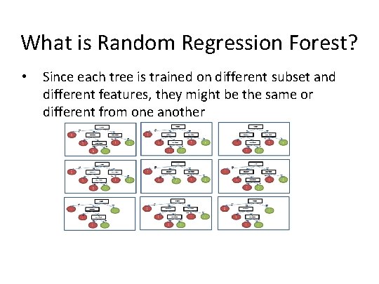
What is Random Regression Forest? • Since each tree is trained on different subset and different features, they might be the same or different from one another

What is Random Regression Forest? • One prediction per input per tree, the final prediction: – nominal class (decision forest): majority votes – numeric class (regression forest): average prediction • Advantage of random forest: – Smaller training set per tree = smaller prediction variance – Less overfitting than trees • Refer to reference [2] for more details

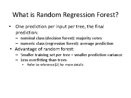
Random Forest in This Application • Each tree is trained on a set of patches randomly sampled from training set • The data are all images, the “features” are totally different from the “obvious” features, such as weather=sunny. – How do they use the image to construct the tree? Image taken from [1]

What They Actually Do • Map of Image Channels i. e. depth, x, y, z 3 5 9 7 11 13 25 35 7 22 30 35 35 40 30 32 11 22 33 44 55 66 77 88 15 30 45 30 32 64 23 12 12 13 15 15 12 13 35 45 43 23 95 65 43 21 23 56 75 93 65 32 21 43 56 58 43 21 65 47 95 23

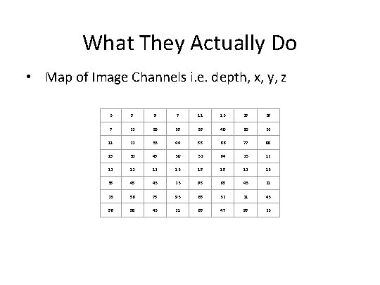
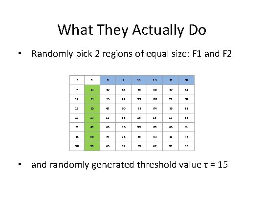
What They Actually Do • Randomly pick 2 regions of equal size: F 1 and F 2 3 5 9 7 11 13 25 35 7 22 30 35 35 40 30 32 11 22 33 44 55 66 77 88 15 30 45 30 32 64 23 12 12 13 15 15 12 13 35 45 43 23 95 65 43 21 23 56 75 93 65 32 21 43 56 58 43 21 65 47 95 23 • and randomly generated threshold value τ = 15

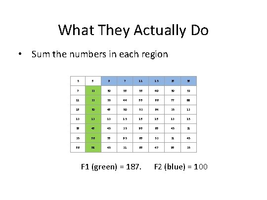
What They Actually Do • Sum the numbers in each region 3 5 9 7 11 13 25 35 7 22 30 35 35 40 30 32 11 22 33 44 55 66 77 88 15 30 45 30 32 64 23 12 12 13 15 15 12 13 35 45 43 23 95 65 43 21 23 56 75 93 65 32 21 43 56 58 43 21 65 47 95 23 F 1 (green) = 187. F 2 (blue) = 100

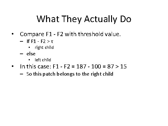
What They Actually Do • Compare F 1 - F 2 with threshold value. – If F 1 - F 2 > τ • right child – else • left child • In this case: F 1 - F 2 = 187 - 100 = 87 > 15 – So this patch belongs to the right child

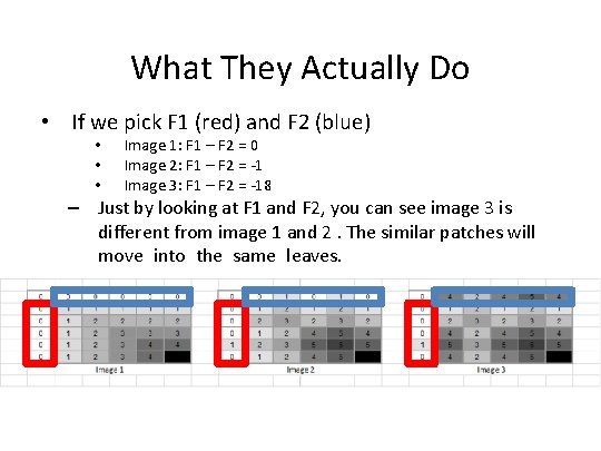
What They Actually Do • If we pick F 1 (red) and F 2 (blue) • • • Image 1: F 1 – F 2 = 0 Image 2: F 1 – F 2 = -1 Image 3: F 1 – F 2 = -18 – Just by looking at F 1 and F 2, you can see image 3 is different from image 1 and 2. The similar patches will move into the same leaves.

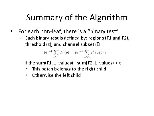
Summary of the Algorithm • For each non-leaf, there is a “binary test” – Each binary test is defined by: regions (F 1 and F 2), threshold (τ), and channel subset (I) – If the sum(F 1. I_values) - sum(F 2. I_values) > τ • This patch belongs to the right child • Otherwise the left child

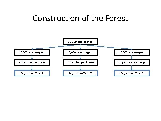
Construction of the Forest 50, 000 face images 3, 000 face images 25 patches per image Regression Tree 1 Regression Tree 2 Regression Tree 3

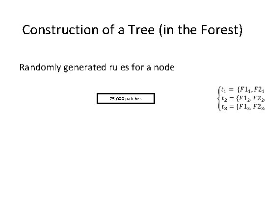
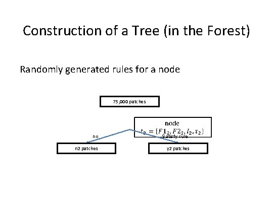
Construction of a Tree (in the Forest) Randomly generated rules for a node 75, 000 patches

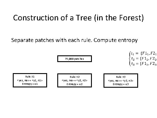
Construction of a Tree (in the Forest) Separate patches with each rule. Compute entropy 75, 000 patches Rule: t 1 <yes, no> = <y 1, n 1> Entropy = e 1 Rule: t 2 <yes, no> = <y 2, n 2> Entropy = e 2 Rule: t 3 <yes, no> = <y 3, n 3> Entropy = e 3

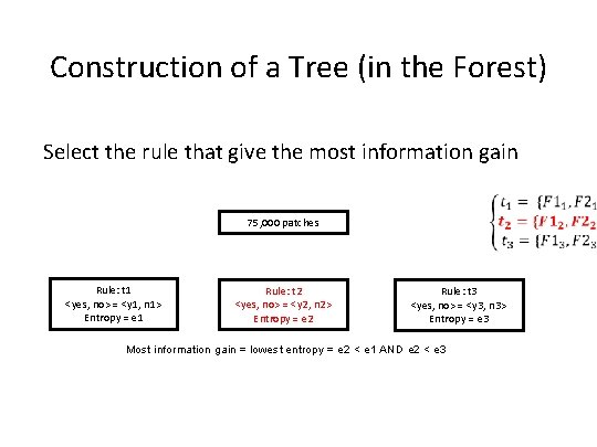
Construction of a Tree (in the Forest) Select the rule that give the most information gain 75, 000 patches Rule: t 1 <yes, no> = <y 1, n 1> Entropy = e 1 Rule: t 2 <yes, no> = <y 2, n 2> Entropy = e 2 Rule: t 3 <yes, no> = <y 3, n 3> Entropy = e 3 Most information gain = lowest entropy = e 2 < e 1 AND e 2 < e 3

Construction of a Tree (in the Forest) Randomly generated rules for a node 75, 000 patches no n 2 patches Satisfy rule y 2 patches

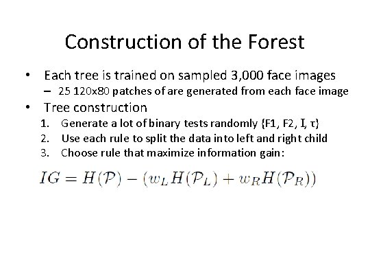
Construction of the Forest • Each tree is trained on sampled 3, 000 face images – 25 120 x 80 patches of are generated from each face image • Tree construction 1. Generate a lot of binary tests randomly {F 1, F 2, I, τ} 2. Use each rule to split the data into left and right child 3. Choose rule that maximize information gain:

Construction of the Forest • Image taken from [1] http: //www. mathworks. com/help/stats/multivariat e-normal-distribution. html

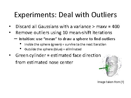
Experiments: Deal with Outliers • Discard all Gaussians with a variance > maxv = 400 • Remove outliers using 10 mean-shift iterations – Intuition: use “mean” to draw a sphere to find outliers • • Inside the sphere (green) = survive to the next iteration Outside the sphere (blue) = eliminated • Green cylinder = estimated face direction from estimated nose center Image taken from [1]

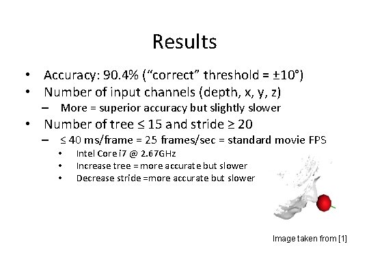
Results • Accuracy: 90. 4% (“correct” threshold = ± 10°) • Number of input channels (depth, x, y, z) – More = superior accuracy but slightly slower • Number of tree ≤ 15 and stride ≥ 20 – ≤ 40 ms/frame = 25 frames/sec = standard movie FPS • • • Intel Core i 7 @ 2. 67 GHz Increase tree = more accurate but slower Decrease stride =more accurate but slower Image taken from [1]

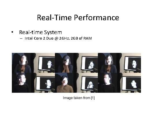
Real-Time Performance • Real-time System – Intel Core 2 Duo @ 2 GHz. 2 GB of RAM Image taken from [1]

Discussion • Did they do as they claim? – Real-time • Number of tree ≤ 15 and stride ≥ 20 – Accuracy • 90. 4% with 10° threshold • 6. 5%: all votes are deleted by mean-shift – In real-time system, video feed is 25 frames/seconds – There a lot of room for error correction

Question and Answer

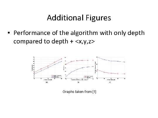
Additional Figures • Performance of the algorithm with only depth compared to depth + <x, y, z> Graphs taken from [1]