Decision Trees CS 548 Fall 2016 Decision Tree

Decision Trees CS 548 Fall 2016 Decision Tree Showcase by Muyeedul Hoque, Chao Xu, Yue Zhao, and Kevin Heath Showcasing work by N. Morizet, N. Godin, J. Tang, E. Maillet, M. Fregonese, and B. Normand on "Classification of Acoustic Emission Signals Using Wavelets and Random Forests: Application to localized corrosion".

References James, G. , Witten, D. , Hastie, T. , & Tibshirani, R. , An Introduction to Statistical Learning. Springer. (2015). Morizet, N. , Godin, N. , Tang, N. , Maillet, E. , Fregonese, M. , & Normand, B. , Classification of Acoustic Emission Signals Using Wavelets and Random Forests: Application to localized corrosion. Mechanical Systems and Signal Processing (2016), 1026 -1037. T. Cover, P. Hart , Nearest neighbor pattern classification, IEEETrans. Inf. Theory 13 (1967), 21– 27. S. Arlot, A. Celisse, A survey of cross-validation procedures for model selection, Stat. Surv. 4 (2010), 40– 79. Wavelet. Retrieved from Wikipedia: https: //en. wikipedia. org/wiki/Wavelet (2016, September 10). T. F. Barton, D. L. Tuck, D. B. Wells, The identification of pitting and crevice corrosion spectra in electrochemical noise using an artificial neural network, in: ASTM Special Technical Publication, vol. 1277 (1996), pp. 157– 169. R. Piotrkowski, E. Castro, A. Gallego, Wavelet power, entropy and bispectrum applied to ae signals for damage identification and evaluation of corroded galvanized steel, Mech. Syst. Signal Process. 23 (2009), 432– 445. J. Griffin, X. Chen, Multiple classification of the acoustic emission signals extracted during burn and chatter anomalies using genetic programming, Int. J. Adv. Manuf. Technol. 45 (2009), 1152– 1168. Y. Yu, L. Zhou, Acoustic emission signal classification based on support vector machine, TELKOMNIKA : Indones. J. Electr. Eng. 10 (2012), 1027– 1032.

Agenda • Introduction to Acoustic Emission Signals • Feature extraction from preprocessed waveforms • Supervised classification using random forests • Ground Truth and Tests • Conclusion

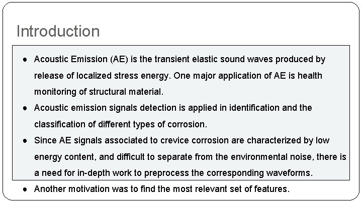
Introduction ● Acoustic Emission (AE) is the transient elastic sound waves produced by release of localized stress energy. One major application of AE is health monitoring of structural material. ● Acoustic emission signals detection is applied in identification and the classification of different types of corrosion. ● Since AE signals associated to crevice corrosion are characterized by low energy content, and difficult to separate from the environmental noise, there is a need for in-depth work to preprocess the corresponding waveforms. ● Another motivation was to find the most relevant set of features.

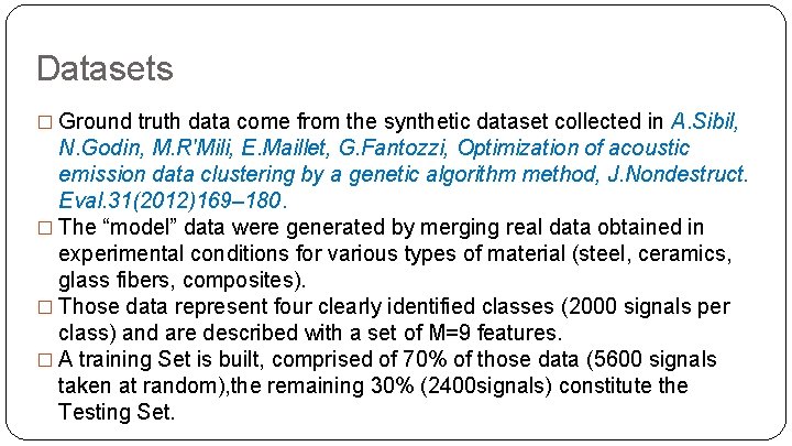
Datasets � Ground truth data come from the synthetic dataset collected in A. Sibil, N. Godin, M. R'Mili, E. Maillet, G. Fantozzi, Optimization of acoustic emission data clustering by a genetic algorithm method, J. Nondestruct. Eval. 31(2012)169– 180. � The “model” data were generated by merging real data obtained in experimental conditions for various types of material (steel, ceramics, glass fibers, composites). � Those data represent four clearly identified classes (2000 signals per class) and are described with a set of M=9 features. � A training Set is built, comprised of 70% of those data (5600 signals taken at random), the remaining 30% (2400 signals) constitute the Testing Set.

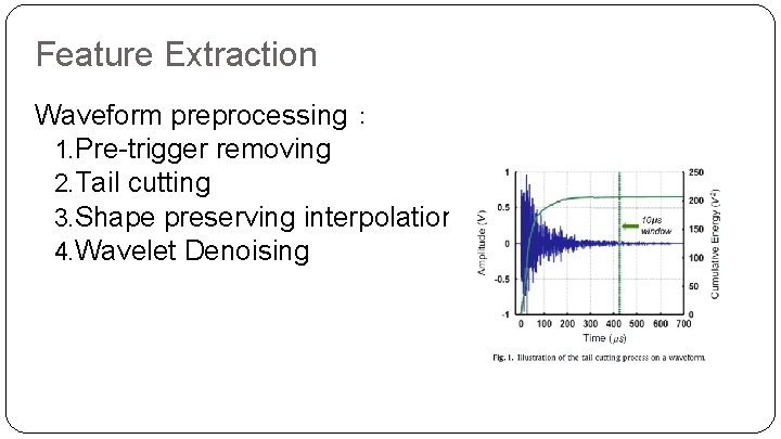
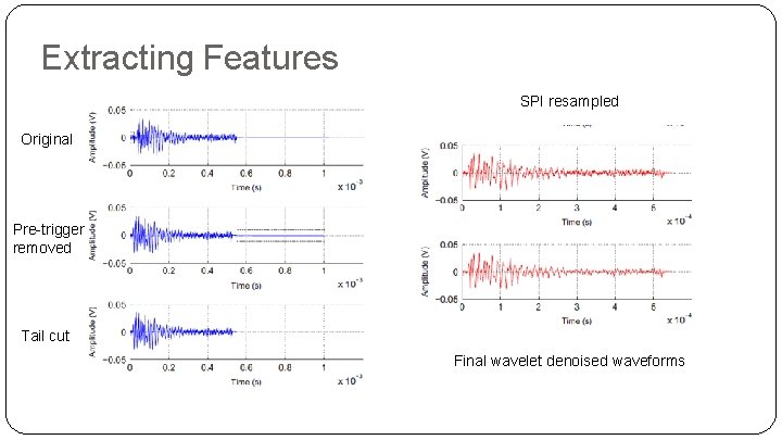
Feature Extraction Waveform preprocessing： 1. Pre-trigger removing 2. Tail cutting 3. Shape preserving interpolation (SPI) resampling 4. Wavelet Denoising

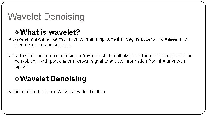
Wavelet Denoising ❖What is wavelet? A wavelet is a wave-like oscillation with an amplitude that begins at zero, increases, and then decreases back to zero. Wavelets can be combined, using a "reverse, shift, multiply and integrate" technique called convolution, with portions of a known signal to extract information from the unknown signal. ❖Wavelet Denoising wden function from the Matlab Wavelet Toolbox

Extracting Features SPI resampled Original Pre-trigger removed Tail cut Final wavelet denoised waveforms

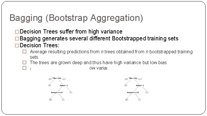
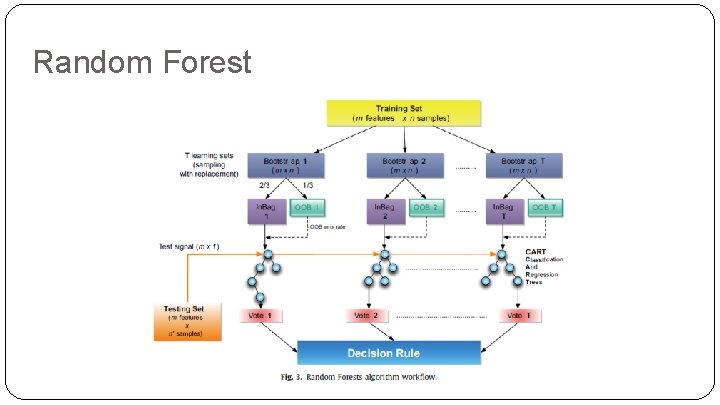
Bagging (Bootstrap Aggregation) �Decision Trees suffer from high variance �Bagging generates several different Bootstrapped training sets �Decision Trees: � Average resulting predictions from n trees obtained from n bootstrapped training sets � The trees are grown deep and thus have high variance but low bias � Averaging the trees leads to low variance

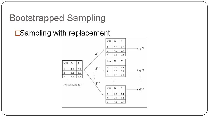
Bootstrapped Sampling �Sampling with replacement

Bagging – Out-of-Bag Error Estimation � Each bagged tree tends to use 2/3 rd of all observations � Remaining 1/3 rd – OOB observations � Test Error – Average B/3 predictions � Overall, Bagging improves accuracy but loses on interpretability � For Prediction: � MV - Majority vote among all B trees � Security Vote (SV) - if more than 70% voted for a specific class

Random Forest �Random Forest utilizes Bagging techniques, but de-correlates trees �Each time a tree is split, a random sample of m predictors is chosen � m is usually √(total number of predictors) �Otherwise, all trees may use key predictor(s) � Trees will then be highly correlated, not reducing variance. �If m = total number of predictors, then random forest essentially runs bagging.

Random Forest

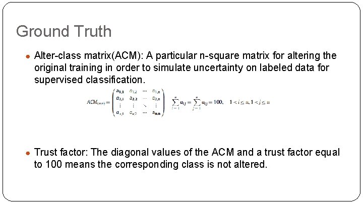
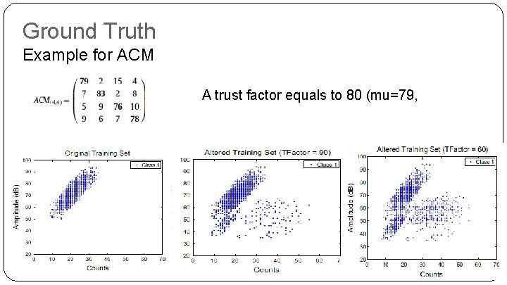
Ground Truth ● Alter-class matrix(ACM): A particular n-square matrix for altering the original training in order to simulate uncertainty on labeled data for supervised classification. ● Trust factor: The diagonal values of the ACM and a trust factor equal to 100 means the corresponding class is not altered.

Ground Truth Example for ACM A trust factor equals to 80 (mu=79, sigma=2. 94)

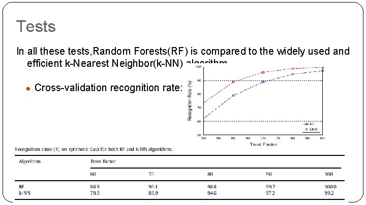
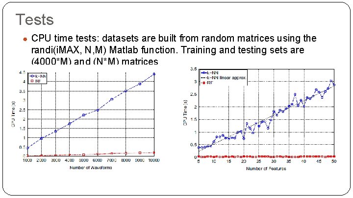
Tests In all these tests, Random Forests(RF) is compared to the widely used and efficient k-Nearest Neighbor(k-NN) algorithm. ● Cross-validation recognition rate:

Tests ● CPU time tests: datasets are built from random matrices using the randi(i. MAX, N, M) Matlab function. Training and testing sets are (4000*M) and (N*M) matrices

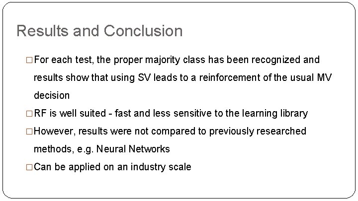
Results and Conclusion �For each test, the proper majority class has been recognized and results show that using SV leads to a reinforcement of the usual MV decision �RF is well suited - fast and less sensitive to the learning library �However, results were not compared to previously researched methods, e. g. Neural Networks �Can be applied on an industry scale