CPSC 641 Network Traffic SelfSimilarity Carey Williamson Department

CPSC 641: Network Traffic Self-Similarity Carey Williamson Department of Computer Science University of Calgary

Introduction § A classic network traffic measurement study has shown that aggregate Ethernet LAN traffic is self-similar [Leland et al 1993] § A statistical property that is very different from the traditional Poisson-based models § This presentation: definition of network traffic selfsimilarity, Bellcore Ethernet LAN data, implications of self-similarity

Measurement Methodology § Collected lengthy traces of Ethernet LAN traffic on Ethernet LAN(s) at Bellcore § High resolution time stamps § Analyzed statistical properties of the resulting time series data § Each observation represents the number of packets (or bytes) observed per time interval (e. g. , 10 4 8 12 7 2 0 5 17 9 8 8 2. . . )

Self-Similarity: The Intuition § If you plot the number of packets observed per time interval as a function of time, then the plot looks ‘‘similar’’ regardless of what interval size you choose § E. g. , 10 msec, 100 msec, 10 sec, . . . § Same applies if you plot number of bytes observed per interval of time

Self-Similarity: The Intuition § In other words, self-similarity implies a ‘‘fractallike’’ behaviour: no matter what time scale you use to examine the data, you see similar patterns § Implications: — Burstiness exists across many time scales — No natural length of a burst — Traffic does not necessarilty get ‘‘smoother” when you aggregate it (unlike Poisson traffic)

Self-Similarity: The Mathematics § Self-similarity is a rigourous statistical property (i. e. , a lot more to it than just the pretty ‘‘fractallike’’ pictures) § Assumes you have time series data with finite mean and variance (i. e. , covariance stationary stochastic process) § Must be a very long time series (infinite is best!) § Can test for presence of self-similarity

Self-Similarity: The Mathematics § Self-similarity manifests itself in several equivalent fashions: § Slowly decaying variance § Long range dependence § Non-degenerate autocorrelations § Hurst effect

Slowly Decaying Variance § The variance of the sample decreases more slowly than the reciprocal of the sample size § For most processes, the variance of a sample diminishes quite rapidly as the sample size is increased, and stabilizes soon § For self-similar processes, the variance decreases very slowly, even when the sample size grows quite large

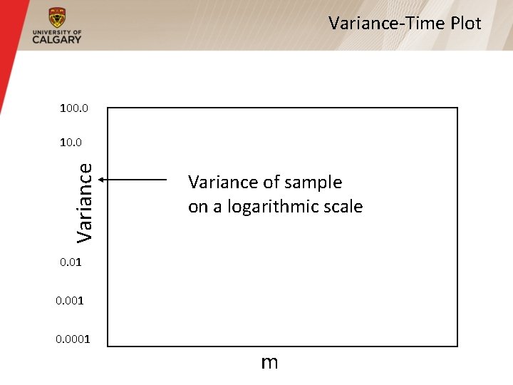
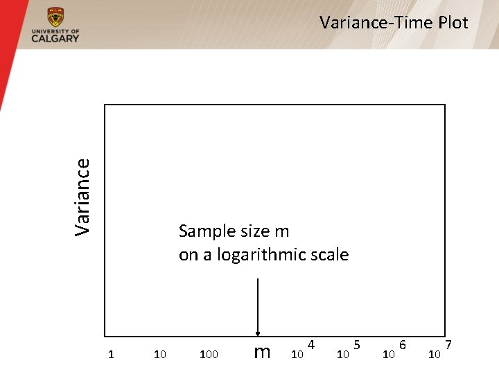
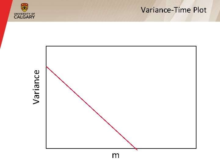
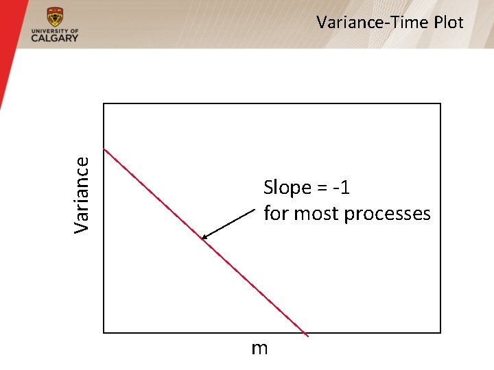
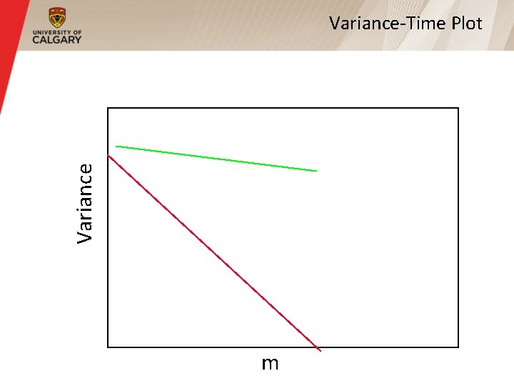
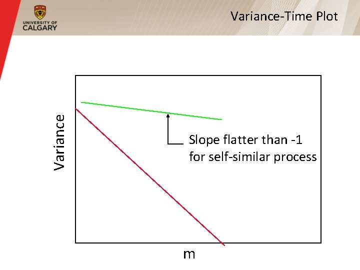
Variance-Time Plot § The ‘‘variance-time plot” is one method to test for the slowly decaying variance property § Plots the variance of the sample versus the sample size, on a log-log plot § For most processes, the result is a straight line with slope -1 § For self-similar, the line is much flatter

Variance-Time Plot m

Variance-Time Plot 100. 0 Variance 10. 0 Variance of sample on a logarithmic scale 0. 01 0. 0001 m

Variance-Time Plot Sample size m on a logarithmic scale 1 10 100 m 10 4 10 5 10 6 10 7

Variance-Time Plot m

Variance-Time Plot m

Variance-Time Plot Slope = -1 for most processes m

Variance-Time Plot m

Variance-Time Plot Slope flatter than -1 for self-similar process m

Long Range Dependence § Correlation is a statistical measure of the relationship, if any, between two random variables § Positive correlation: both behave similarly § Negative correlation: behave in opposite fashion § No correlation: behaviour of one is statistically unrelated to behaviour of other

Long Range Dependence (Cont’d) § Autocorrelation is a statistical measure of the relationship, if any, between a random variable and itself, at different time lags § Positive correlation: big observation usually followed by another big, or small by small § Negative correlation: big observation usually followed by small, or small by big § No correlation: observations unrelated

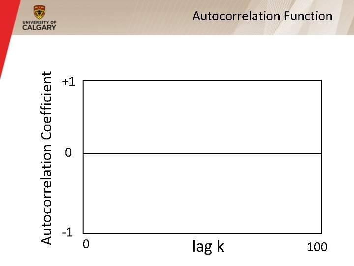
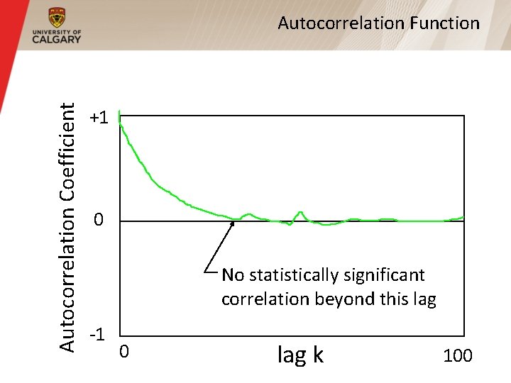
Long Range Dependence (Cont’d) § Autocorrelation coefficient can range between +1 (very high positive correlation) and -1 (very high negative correlation) § Zero means no correlation § Autocorrelation function shows the value of the autocorrelation coefficient for different time lags k

Autocorrelation Coefficient Autocorrelation Function +1 0 -1 0 lag k 100

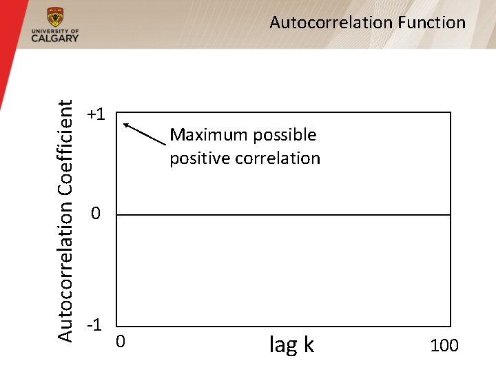
Autocorrelation Coefficient Autocorrelation Function +1 Maximum possible positive correlation 0 -1 0 lag k 100

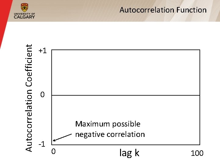
Autocorrelation Coefficient Autocorrelation Function +1 0 -1 Maximum possible negative correlation 0 lag k 100

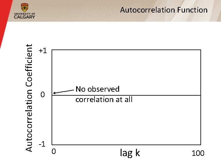
Autocorrelation Coefficient Autocorrelation Function +1 No observed correlation at all 0 -1 0 lag k 100

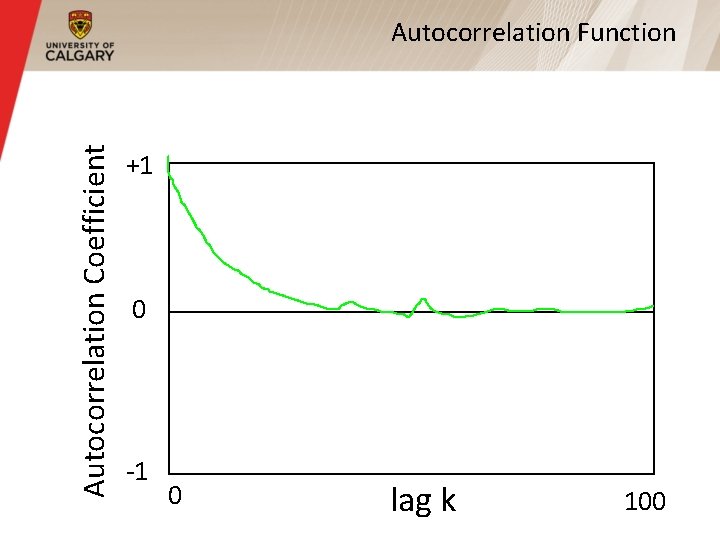
Autocorrelation Coefficient Autocorrelation Function +1 0 -1 0 lag k 100

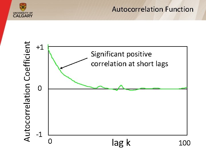
Autocorrelation Coefficient Autocorrelation Function +1 Significant positive correlation at short lags 0 -1 0 lag k 100

Autocorrelation Coefficient Autocorrelation Function +1 0 No statistically significant correlation beyond this lag -1 0 lag k 100

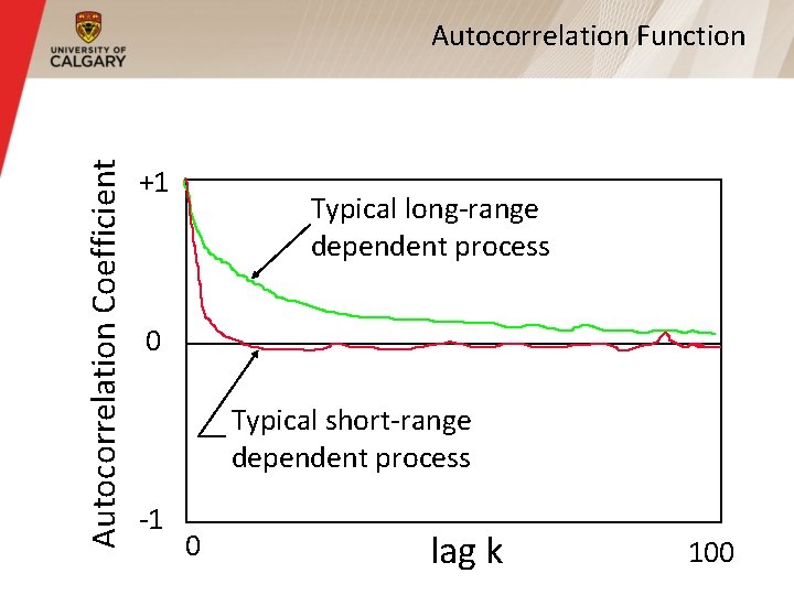
Long Range Dependence (Cont’d) § For most processes (e. g. , Poisson, or compound Poisson), the autocorrelation function drops to zero very quickly (usually immediately, or exponentially fast) § For self-similar processes, the autocorrelation function drops very slowly (i. e. , hyperbolically) toward zero, but may never reach zero § Non-summable autocorrelation function

Autocorrelation Coefficient Autocorrelation Function +1 Typical long-range dependent process 0 Typical short-range dependent process -1 0 lag k 100

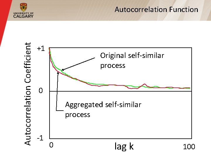
Non-Degenerate Autocorrelations § For self-similar processes, the autocorrelation function for the aggregated process is indistinguishable from that of the original process § If autocorrelation coefficients match for all lags k, then called exactly self-similar § If autocorrelation coefficients match only for large lags k, then called asymptotically self-similar

Autocorrelation Coefficient Autocorrelation Function +1 Original self-similar process 0 Aggregated self-similar process -1 0 lag k 100

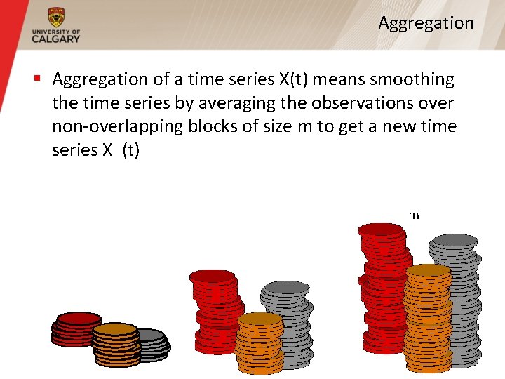
Aggregation § Aggregation of a time series X(t) means smoothing the time series by averaging the observations over non-overlapping blocks of size m to get a new time series X (t) m

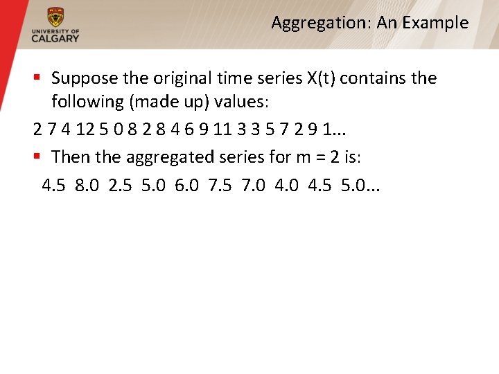
Aggregation: An Example § Suppose the original time series X(t) contains the following (made up) values: 2 7 4 12 5 0 8 2 8 4 6 9 11 3 3 5 7 2 9 1. . . § Then the aggregated series for m = 2 is:

Aggregation: An Example § Suppose the original time series X(t) contains the following (made up) values: 2 7 4 12 5 0 8 2 8 4 6 9 11 3 3 5 7 2 9 1. . . § Then the aggregated series for m = 2 is: 4. 5 8. 0 2. 5 5. 0 6. 0 7. 5 7. 0 4. 5 5. 0. . .

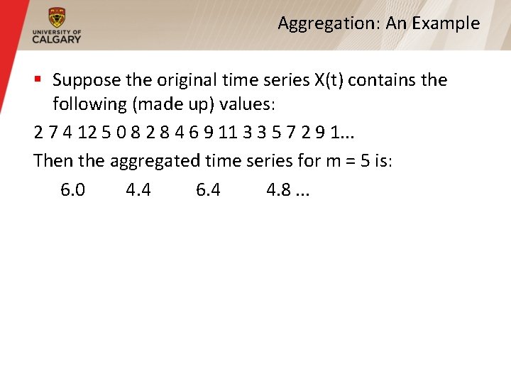
Aggregation: An Example § Suppose the original time series X(t) contains the following (made up) values: 2 7 4 12 5 0 8 2 8 4 6 9 11 3 3 5 7 2 9 1. . . Then the aggregated time series for m = 5 is:

Aggregation: An Example § Suppose the original time series X(t) contains the following (made up) values: 2 7 4 12 5 0 8 2 8 4 6 9 11 3 3 5 7 2 9 1. . . Then the aggregated time series for m = 5 is: 6. 0 4. 4 6. 4 4. 8. . .

Autocorrelation Coefficient Autocorrelation Function +1 Original self-similar process 0 Aggregated self-similar process -1 0 lag k 100

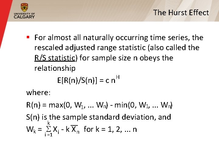
The Hurst Effect § For almost all naturally occurring time series, the rescaled adjusted range statistic (also called the R/S statistic) for sample size n obeys the relationship H E[R(n)/S(n)] = c n where: R(n) = max(0, W 1, . . . Wn) - min(0, W 1, . . . Wn) S(n) is the sample standard deviation, and k Wk = X i - k Xn for k = 1, 2, . . . n i =1

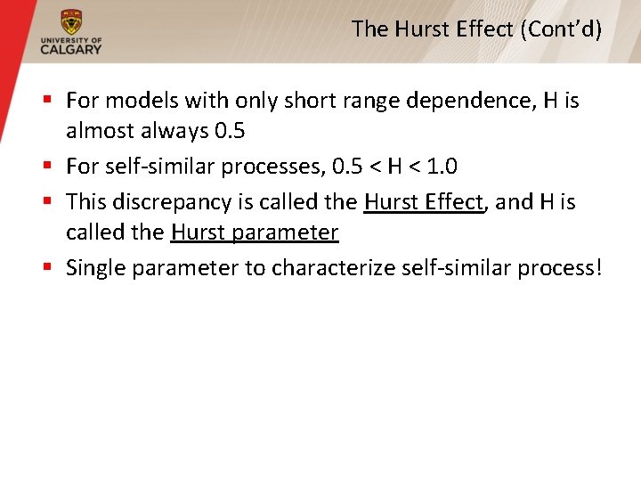
The Hurst Effect (Cont’d) § For models with only short range dependence, H is almost always 0. 5 § For self-similar processes, 0. 5 < H < 1. 0 § This discrepancy is called the Hurst Effect, and H is called the Hurst parameter § Single parameter to characterize self-similar process!

R/S Statistic: An Example § Suppose the original time series X(t) contains the following (made up) values: 2 7 4 12 5 0 8 2 8 4 6 9 11 3 3 5 7 2 9 1 § There are 20 data points in this example

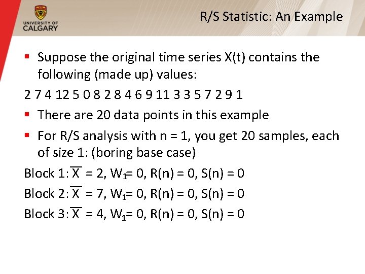
R/S Statistic: An Example § Suppose the original time series X(t) contains the following (made up) values: 2 7 4 12 5 0 8 2 8 4 6 9 11 3 3 5 7 2 9 1 § There are 20 data points in this example § For R/S analysis with n = 1, you get 20 samples, each of size 1: (boring base case) Block 1: X = 2, W 1= 0, R(n) = 0, S(n) = 0 Block 2: X = 7, W 1= 0, R(n) = 0, S(n) = 0 Block 3: X = 4, W 1= 0, R(n) = 0, S(n) = 0

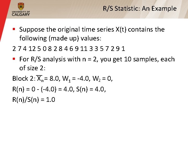
R/S Statistic: An Example § Suppose the original time series X(t) contains the following (made up) values: 2 7 4 12 5 0 8 2 8 4 6 9 11 3 3 5 7 2 9 1 § For R/S analysis with n = 2, you get 10 samples, each of size 2:

R/S Statistic: An Example § Suppose the original time series X(t) contains the following (made up) values: 2 7 4 12 5 0 8 2 8 4 6 9 11 3 3 5 7 2 9 1 § For R/S analysis with n = 2, you get 10 samples, each of size 2: Block 1: Xn = 4. 5, W 1 = -2. 5, W 2 = 0, R(n) = 0 - (-2. 5) = 2. 5, S(n) = 2. 5, R(n)/S(n) = 1. 0

R/S Statistic: An Example § Suppose the original time series X(t) contains the following (made up) values: 2 7 4 12 5 0 8 2 8 4 6 9 11 3 3 5 7 2 9 1 § For R/S analysis with n = 2, you get 10 samples, each of size 2: Block 2: Xn = 8. 0, W 1 = -4. 0, W 2 = 0, R(n) = 0 - (-4. 0) = 4. 0, S(n) = 4. 0, R(n)/S(n) = 1. 0

R/S Statistic: An Example § Suppose the original time series X(t) contains the following (made up) values: 2 7 4 12 5 0 8 2 8 4 6 9 11 3 3 5 7 2 9 1 § For R/S analysis with n = 5, you get 4 samples, each of size 5:

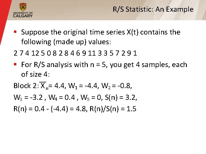
R/S Statistic: An Example § Suppose the original time series X(t) contains the following (made up) values: 2 7 4 12 5 0 8 2 8 4 6 9 11 3 3 5 7 2 9 1 § For R/S analysis with n = 5, you get 4 samples, each of size 4: Block 1: Xn = 6. 0, W 1 = -4. 0, W 2 = -3. 0, W 3 = -5. 0 , W 4 = 1. 0 , W 5 = 0, S(n) = 3. 41, R(n) = 1. 0 - (-5. 0) = 6. 0, R(n)/S(n) = 1. 76

R/S Statistic: An Example § Suppose the original time series X(t) contains the following (made up) values: 2 7 4 12 5 0 8 2 8 4 6 9 11 3 3 5 7 2 9 1 § For R/S analysis with n = 5, you get 4 samples, each of size 4: Block 2: X n= 4. 4, W 1 = -4. 4, W 2 = -0. 8, W 3 = -3. 2 , W 4 = 0. 4 , W 5 = 0, S(n) = 3. 2, R(n) = 0. 4 - (-4. 4) = 4. 8, R(n)/S(n) = 1. 5

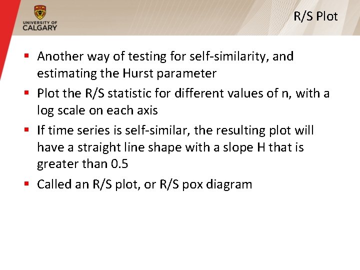
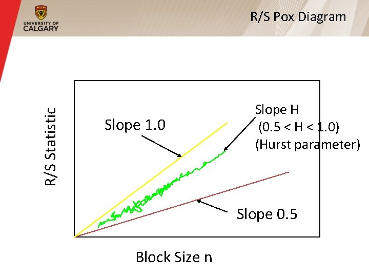
R/S Plot § Another way of testing for self-similarity, and estimating the Hurst parameter § Plot the R/S statistic for different values of n, with a log scale on each axis § If time series is self-similar, the resulting plot will have a straight line shape with a slope H that is greater than 0. 5 § Called an R/S plot, or R/S pox diagram

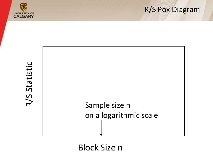
R/S Statistic R/S Pox Diagram Block Size n

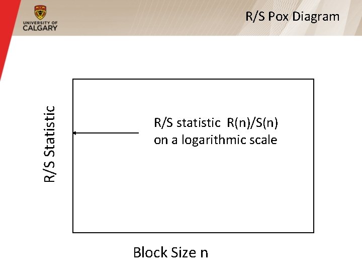
R/S Statistic R/S Pox Diagram R/S statistic R(n)/S(n) on a logarithmic scale Block Size n

R/S Statistic R/S Pox Diagram Sample size n on a logarithmic scale Block Size n

R/S Statistic R/S Pox Diagram Slope 1. 0 Slope H (0. 5 < H < 1. 0) (Hurst parameter) Slope 0. 5 Block Size n

Summary § Self-similarity is an important mathematical property that has been identified as present in network traffic measurements § Important property: burstiness across many time scales, traffic does not aggregate well § There exist several mathematical methods to test for the presence of self-similarity, and to estimate the Hurst parameter H § There exist models for self-similar traffic