CPSC 531 System Modeling and Simulation Carey Williamson

CPSC 531: System Modeling and Simulation Carey Williamson Department of Computer Science University of Calgary Fall 2017

Motivating Quote for Queueing Models “Good things come to those who wait” - poet/writer Violet Fane, 1892 - song lyrics by Nayobe, 1984 - motto for Heinz Ketchup, USA, 1980’s - slogan for Guinness stout, UK, 1990’s 2

Outline: Queueing Models 1. 2. 3. 4. Basic components of a queue General rules Markov models Common queueing models 3

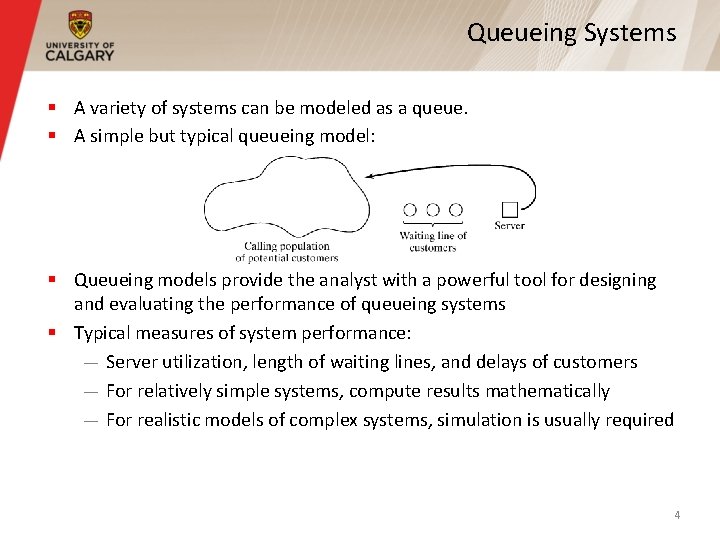
Queueing Systems § A variety of systems can be modeled as a queue. § A simple but typical queueing model: § Queueing models provide the analyst with a powerful tool for designing and evaluating the performance of queueing systems § Typical measures of system performance: — Server utilization, length of waiting lines, and delays of customers — For relatively simple systems, compute results mathematically — For realistic models of complex systems, simulation is usually required 4

Queueing Systems § Key elements of queueing systems: — Customer: refers to anything that arrives at a facility and requires service (e. g. , people, machines, trucks, emails) — Server: refers to any resource that provides the requested service (e. g. , barber, repair person, car wash, file server) 5

Calling Population § Calling population: the population of potential customers, which could be finite or infinite — Finite population model: arrival rate depends on the number of customers in the system, and their current states (e. g. , if you have only one laptop, and it is currently at the repair shop, then the arrival rate of failed laptops from you becomes zero) — Infinite population model: arrival rate is not affected by the number of customers in the system (e. g. , systems with large population of potential customers) 6

System Capacity § System capacity: a limit on the maximum number of customers that may be in service or waiting in line — Limited capacity (e. g. , an automatic car wash only has room for 10 cars to wait in line to enter the wash bay) — Unlimited capacity (e. g. , concert ticket sales with no limit on the number of people allowed to wait to purchase tickets) 7

Queue Behavior and Queue Discipline § Queue behavior: the actions of customers while in a queue waiting for service to begin, for example: — Balk: leave when they see that the line is too long — Renege: leave after being in the line when its moving too slowly — Jockey: move from one line to a shorter line § Queue discipline: the logical ordering of customers in a queue that determines which customer is chosen for service when a server becomes available, for example: — First-in-first-out (FIFO) — Last-in-first-out (LIFO) — Service in random order (SIRO) — Shortest job first (SJF) — Service according to priority (PRI) 8

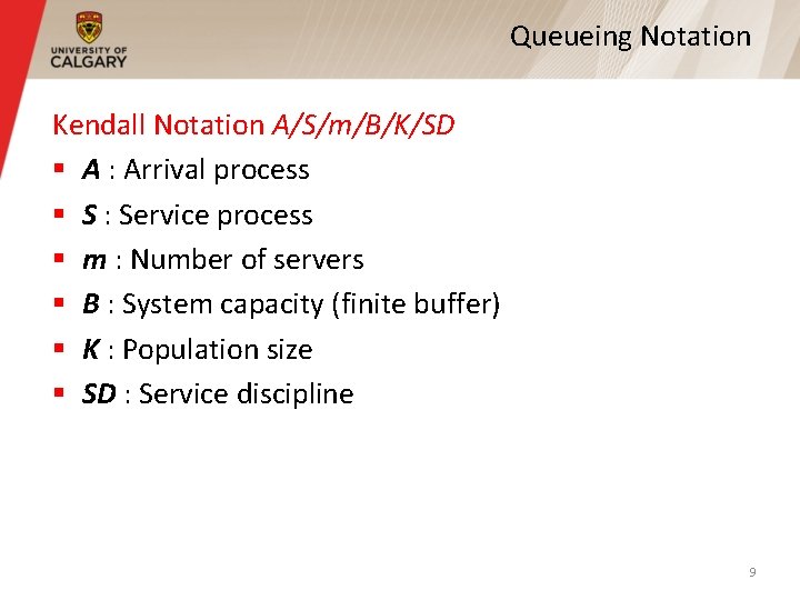
Queueing Notation Kendall Notation A/S/m/B/K/SD § A : Arrival process § S : Service process § m : Number of servers § B : System capacity (finite buffer) § K : Population size § SD : Service discipline 9

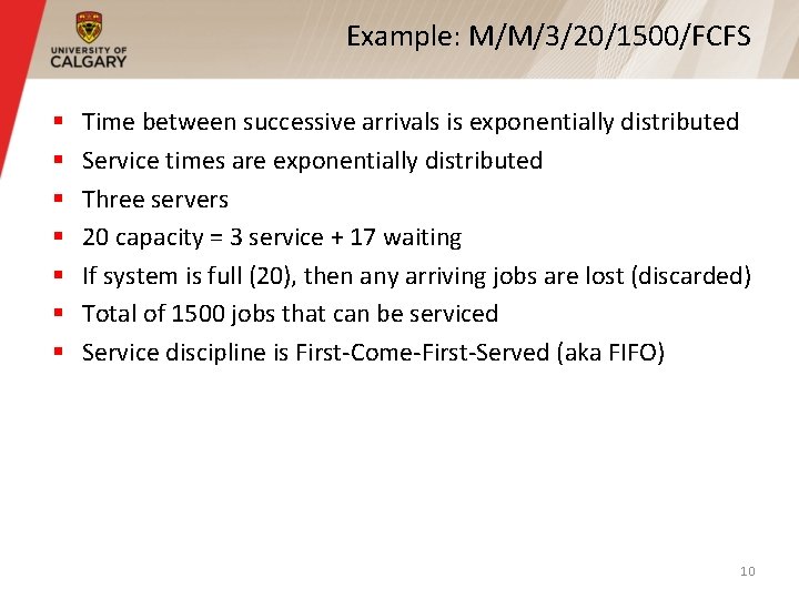
Example: M/M/3/20/1500/FCFS § § § § Time between successive arrivals is exponentially distributed Service times are exponentially distributed Three servers 20 capacity = 3 service + 17 waiting If system is full (20), then any arriving jobs are lost (discarded) Total of 1500 jobs that can be serviced Service discipline is First-Come-First-Served (aka FIFO) 10

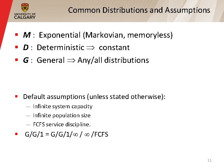
Common Distributions and Assumptions § M : Exponential (Markovian, memoryless) § D : Deterministic constant § G : General Any/all distributions § Default assumptions (unless stated otherwise): — Infinite system capacity — Infinite population size — FCFS service discipline. § G/G/1 = G/G/1/ / /FCFS 11

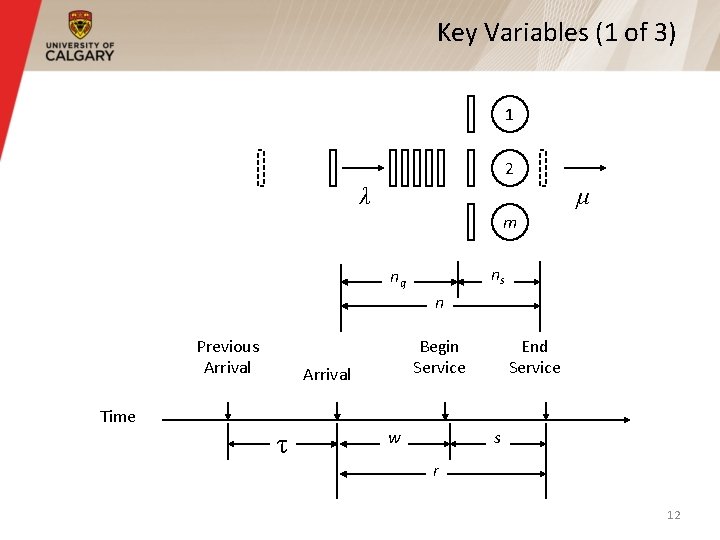
Key Variables (1 of 3) 1 2 λ μ m ns nq n Previous Arrival Begin Service Arrival Time τ w End Service s r 12

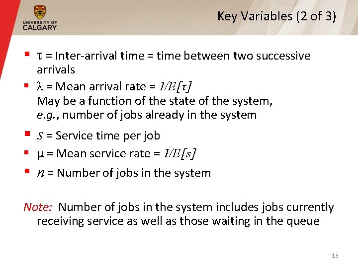
Key Variables (2 of 3) § τ = Inter-arrival time = time between two successive arrivals § λ = Mean arrival rate = 1/E[τ] May be a function of the state of the system, e. g. , number of jobs already in the system § s = Service time per job § μ = Mean service rate = 1/E[s] § n = Number of jobs in the system Note: Number of jobs in the system includes jobs currently receiving service as well as those waiting in the queue 13

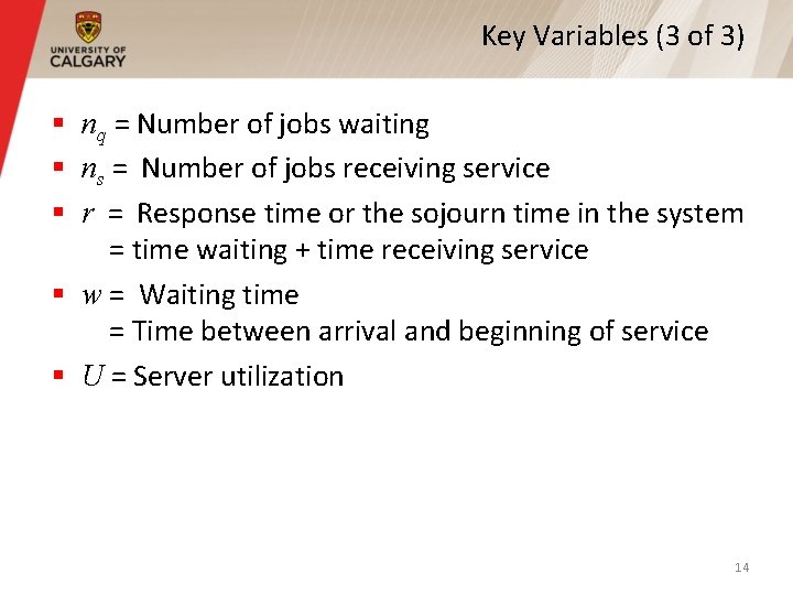
Key Variables (3 of 3) § nq = Number of jobs waiting § ns = Number of jobs receiving service § r = Response time or the sojourn time in the system = time waiting + time receiving service § w = Waiting time = Time between arrival and beginning of service § U = Server utilization 14

Outline 1. 2. 3. 4. Basic components of a queue General rules Markov models Common queueing models 15

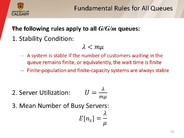
Fundamental Rules for All Queues § 16

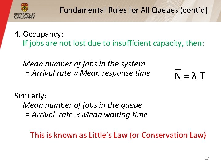
Fundamental Rules for All Queues (cont’d) 4. Occupancy: If jobs are not lost due to insufficient capacity, then: Mean number of jobs in the system = Arrival rate Mean response time N = λ T Similarly: Mean number of jobs in the queue = Arrival rate Mean waiting time This is known as Little’s Law (or Conservation Law) 17

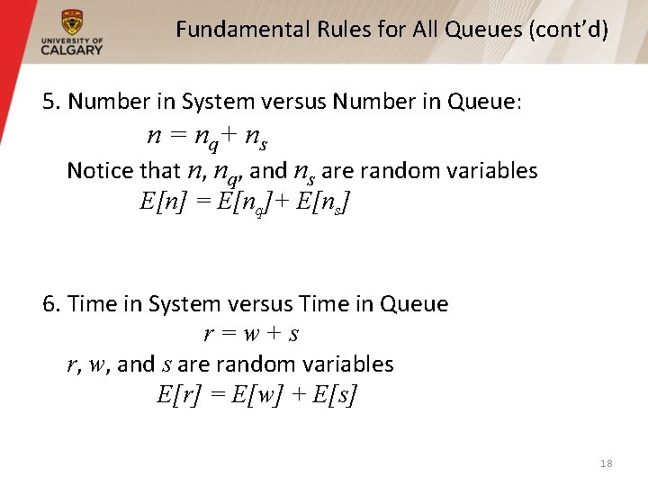
Fundamental Rules for All Queues (cont’d) 5. Number in System versus Number in Queue: n = nq+ ns Notice that n, nq, and ns are random variables E[n] = E[nq]+ E[ns] 6. Time in System versus Time in Queue r = w + s r, w, and s are random variables E[r] = E[w] + E[s] 18

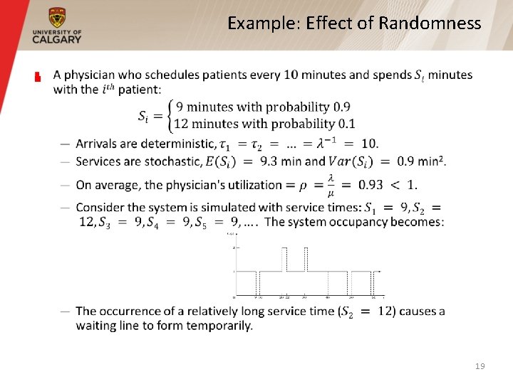
Example: Effect of Randomness § 19

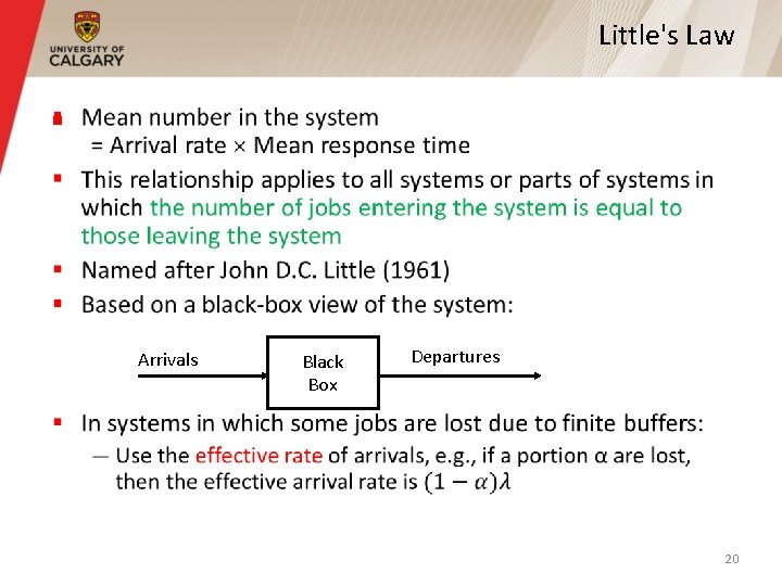
Little's Law § Arrivals Black Box Departures 20

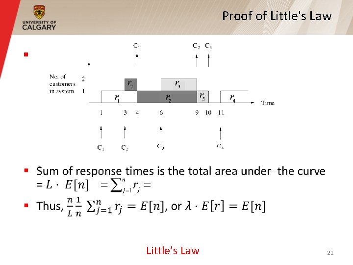
Proof of Little's Law § Little’s Law 21

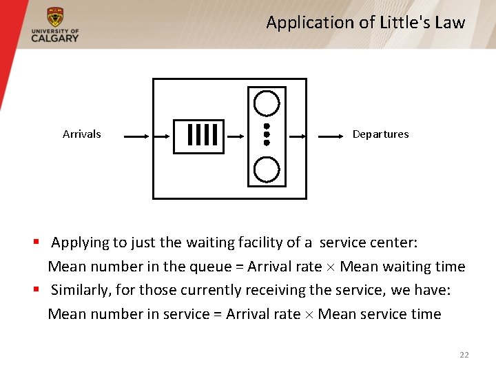
Application of Little's Law Arrivals Departures § Applying to just the waiting facility of a service center: Mean number in the queue = Arrival rate Mean waiting time § Similarly, for those currently receiving the service, we have: Mean number in service = Arrival rate Mean service time 22

Example: I/O System Analysis § A monitor on a disk server showed that the average time to satisfy an I/O request was 100 milliseconds. The I/O rate was about 100 requests per second. What was the mean number of requests at the disk server? § Using Little's law: Mean number at the disk server = Arrival rate Response time = 100 (requests/second) (0. 1 seconds) = 10 requests 23

Some Properties § Utilization factor, throughput, and Little’s formula are not affected by scheduling discipline § Little’s formula can also be applied to an arbitrary queueing system (including queueing networks) 24

Outline 1. 2. 3. 4. Basic components of a queue General rules Markov models Common queueing models 25

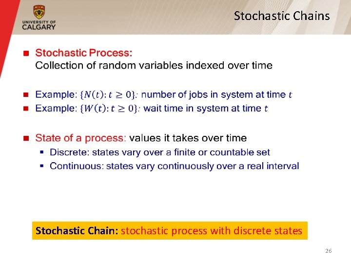
Stochastic Chains § Stochastic Chain: stochastic process with discrete states 26

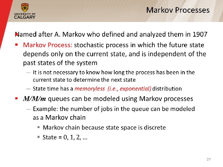
Markov Processes § 27

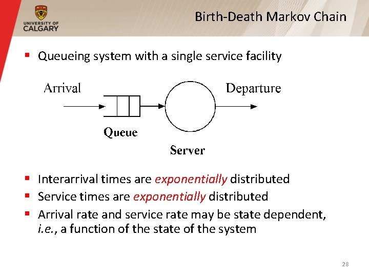
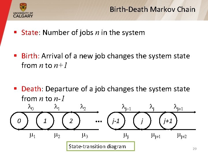
Birth-Death Markov Chain § Queueing system with a single service facility § Interarrival times are exponentially distributed § Service times are exponentially distributed § Arrival rate and service rate may be state dependent, i. e. , a function of the state of the system 28

Birth-Death Markov Chain § State: Number of jobs n in the system § Birth: Arrival of a new job changes the system state from n to n+1 § Death: Departure of a job changes the system state from n to n-1 l 0 0 l 1 1 1 l 2 … 2 2 lj-1 3 j-1 lj j j State-transition diagram lj+1 j+1 j+2 29

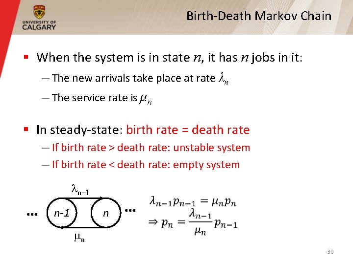
Birth-Death Markov Chain § When the system is in state n, it has n jobs in it: — The new arrivals take place at rate λn — The service rate is μn § In steady-state: birth rate = death rate — If birth rate > death rate: unstable system — If birth rate < death rate: empty system ln-1 … n-1 n … n 30

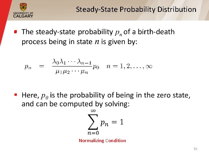
Steady-State Probability Distribution § Normalizing Condition 31

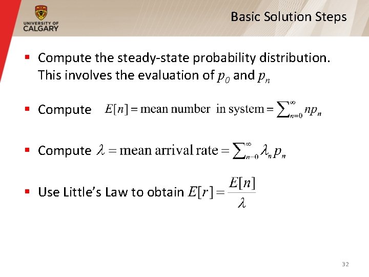
Basic Solution Steps § Compute the steady-state probability distribution. This involves the evaluation of p 0 and pn § Compute § Use Little’s Law to obtain 32

Outline 1. 2. 3. 4. Basic components of a queue General rules Markov models Common queueing models 33

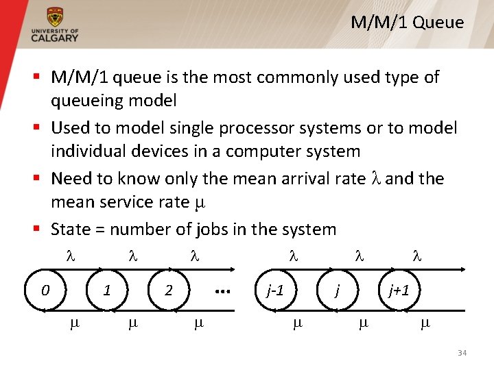
M/M/1 Queue § M/M/1 queue is the most commonly used type of queueing model § Used to model single processor systems or to model individual devices in a computer system § Need to know only the mean arrival rate λ and the mean service rate μ § State = number of jobs in the system l 0 l 1 l … 2 l j-1 l j+1 34

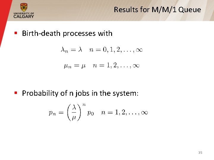
Results for M/M/1 Queue § Birth-death processes with § Probability of n jobs in the system: 35

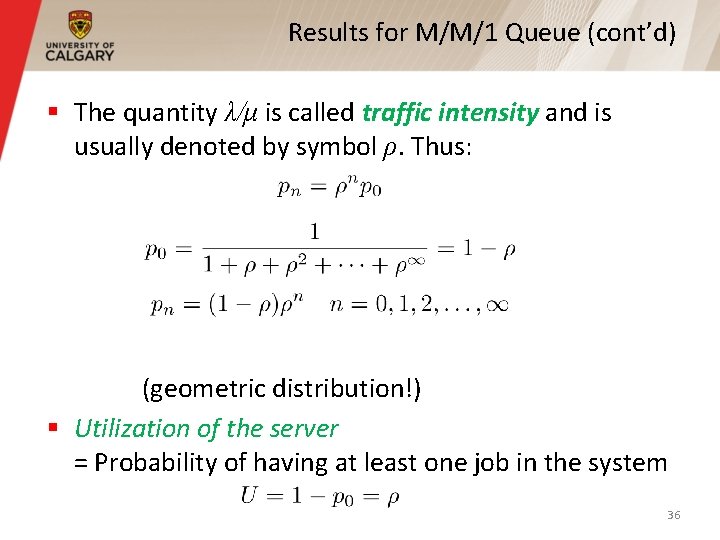
Results for M/M/1 Queue (cont’d) § The quantity λ/μ is called traffic intensity and is usually denoted by symbol ρ. Thus: (geometric distribution!) § Utilization of the server = Probability of having at least one job in the system 36

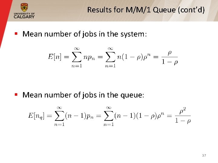
Results for M/M/1 Queue (cont’d) § Mean number of jobs in the system: § Mean number of jobs in the queue: 37

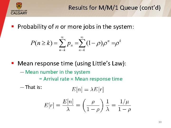
Results for M/M/1 Queue (cont’d) § Probability of n or more jobs in the system: § Mean response time (using Little’s Law): — Mean number in the system = Arrival rate × Mean response time — That is: 38

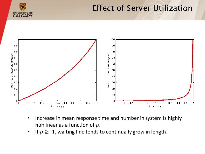
Effect of Server Utilization

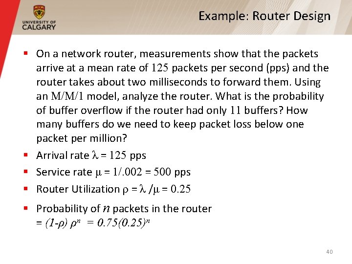
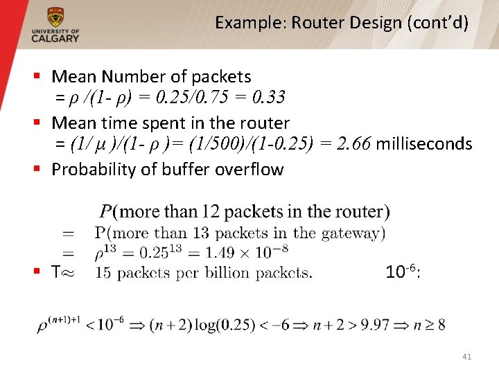
Example: Router Design § On a network router, measurements show that the packets arrive at a mean rate of 125 packets per second (pps) and the router takes about two milliseconds to forward them. Using an M/M/1 model, analyze the router. What is the probability of buffer overflow if the router had only 11 buffers? How many buffers do we need to keep packet loss below one packet per million? § Arrival rate λ = 125 pps § Service rate μ = 1/. 002 = 500 pps § Router Utilization ρ = λ /μ = 0. 25 § Probability of n packets in the router = (1 -ρ) ρn = 0. 75(0. 25)n 40

Example: Router Design (cont’d) § Mean Number of packets = ρ /(1 - ρ) = 0. 25/0. 75 = 0. 33 § Mean time spent in the router = (1/ μ )/(1 - ρ )= (1/500)/(1 -0. 25) = 2. 66 milliseconds § Probability of buffer overflow § To limit the probability of loss to less than 10 -6: 41

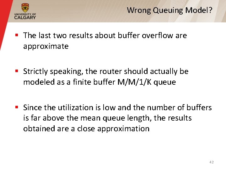
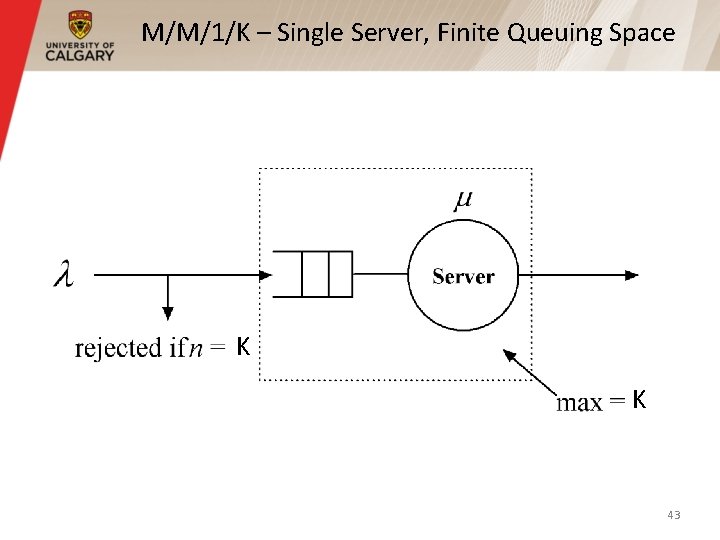
Wrong Queuing Model? § The last two results about buffer overflow are approximate § Strictly speaking, the router should actually be modeled as a finite buffer M/M/1/K queue § Since the utilization is low and the number of buffers is far above the mean queue length, the results obtained are a close approximation 42

M/M/1/K – Single Server, Finite Queuing Space K K 43

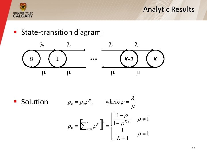
Analytic Results § State-transition diagram: l 0 l … 1 l l K-1 K § Solution 44

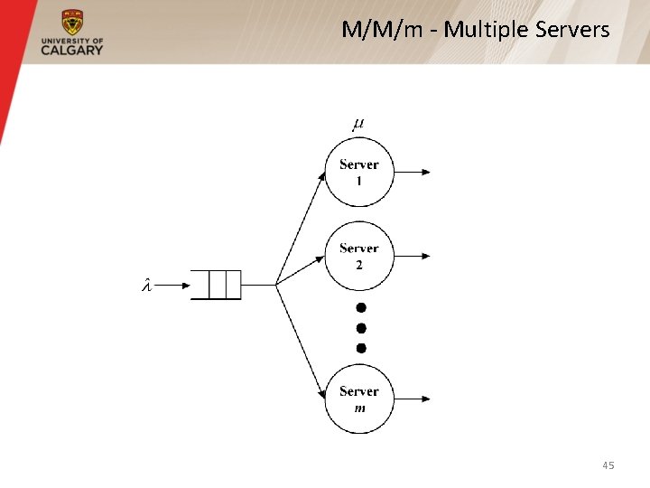
M/M/m - Multiple Servers 45

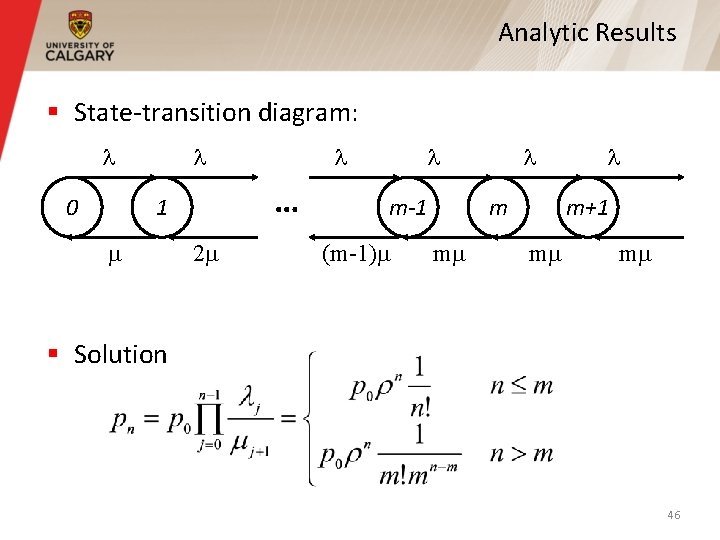
Analytic Results § State-transition diagram: l 0 l … 1 l 2 l m-1 (m-1) l m m l m+1 m m § Solution 46

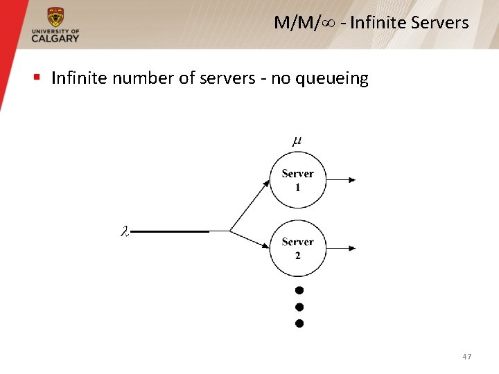
M/M/ - Infinite Servers § Infinite number of servers - no queueing 47

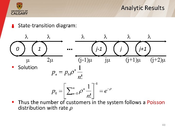
Analytic Results § l 0 l … 1 l 2 l j-1 (j-1) l j j l j+1 (j+1) (j+2) 48

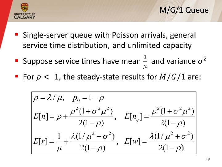
M/G/1 Queue § 49

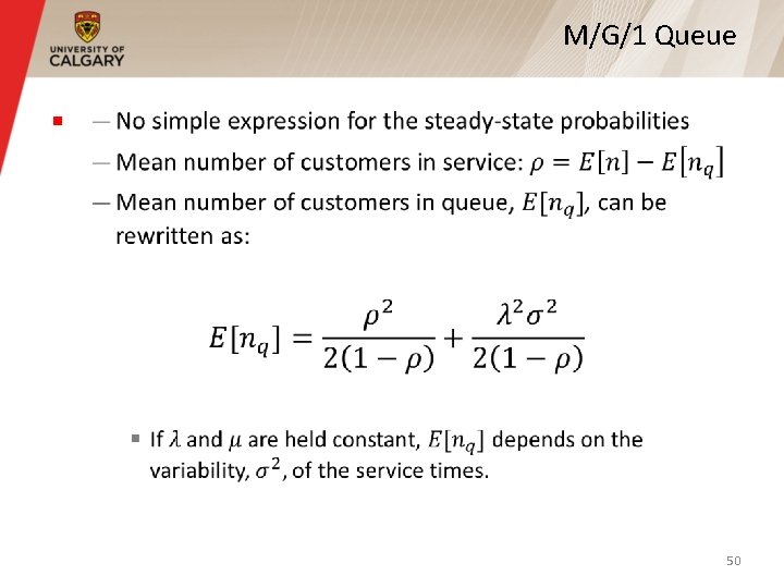
M/G/1 Queue § 50

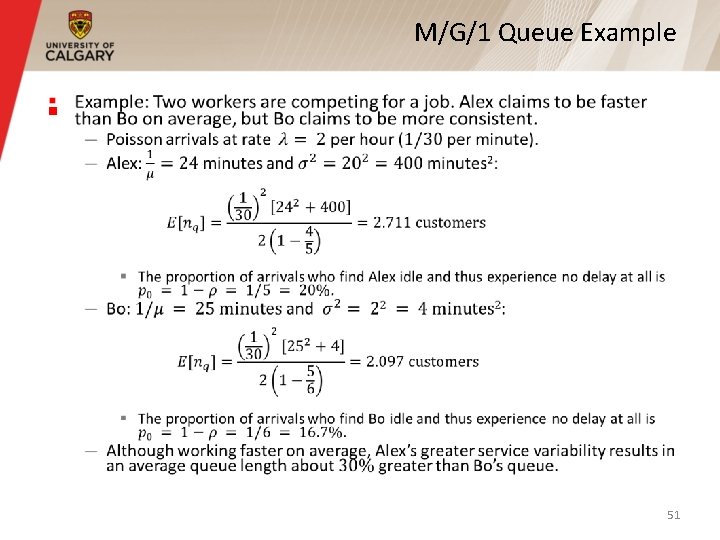
M/G/1 Queue Example § 51

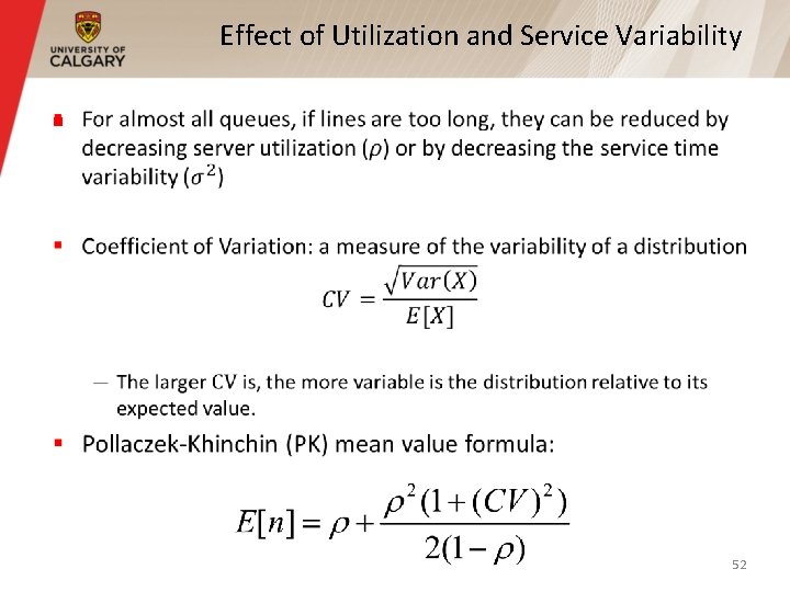
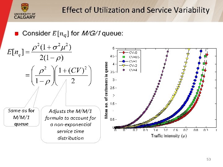
Effect of Utilization and Service Variability § 52

Effect of Utilization and Service Variability Same as for M/M/1 queue Adjusts the M/M/1 formula to account for a non-exponential service time distribution Mean no. of customers in queue § 53