CPSC 531 System Modeling and Simulation Carey Williamson

CPSC 531: System Modeling and Simulation Carey Williamson Department of Computer Science University of Calgary Fall 2017

Statistical Inference § Plan: —Discuss statistical methods in simulations —Define concepts and terminology —Traditional approaches: § Hypothesis testing § Confidence intervals § Batch means § Analysis of Variance (ANOVA)

Motivation § Simulations rely on p. RNG to produce one or more “sample paths” in the stochastic evaluation of a system § Results represent probabilistic answers to the initial perf eval questions of interest § Simulation results must be interpreted accordingly, using the appropriate statistical approaches and methodology

Hypothesis Testing § A technique used to determine whether or not to believe a certain statement (to what degree) § Statement is usually regarding a statistic, and some postulated property of the statistic § Formulate the “null hypothesis” H 0 § Alternative hypothesis H 1 § Decide on statistic to use, and significance level § Collect sample data and calculate test statistic § Decide whether to accept null hypothesis or not

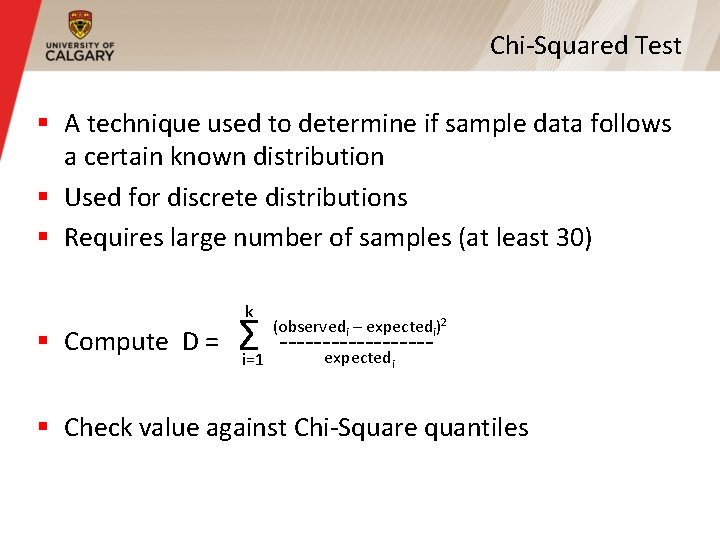
Chi-Squared Test § A technique used to determine if sample data follows a certain known distribution § Used for discrete distributions § Requires large number of samples (at least 30) k § Compute D = Σ i=1 (observedi – expectedi)2 ---------expected i § Check value against Chi-Square quantiles

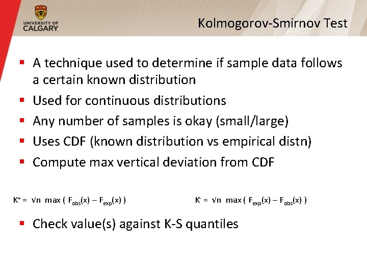
Kolmogorov-Smirnov Test § A technique used to determine if sample data follows a certain known distribution § Used for continuous distributions § Any number of samples is okay (small/large) § Uses CDF (known distribution vs empirical distn) § Compute max vertical deviation from CDF K+ = √n max ( Fobs(x) – Fexp(x) ) K- = √n max ( Fexp(x) – Fobs(x) ) § Check value(s) against K-S quantiles

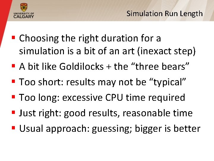
Simulation Run Length § Choosing the right duration for a simulation is a bit of an art (inexact step) § A bit like Goldilocks + the “three bears” § Too short: results may not be “typical” § Too long: excessive CPU time required § Just right: good results, reasonable time § Usual approach: guessing; bigger is better

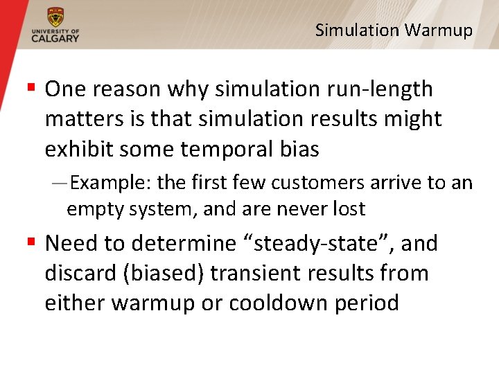
Simulation Warmup § One reason why simulation run-length matters is that simulation results might exhibit some temporal bias —Example: the first few customers arrive to an empty system, and are never lost § Need to determine “steady-state”, and discard (biased) transient results from either warmup or cooldown period

Simulation Replications § One way to establish statistical confidence in simulation results is to repeat an experiment multiple times § Multiple replications, with exact same config parameters, but different seeds § Assumes independent results + normality § Can compute the “mean of means” and the “variance of the global mean”

Statistical Inference § Methods to estimate the characteristics of an entire population based on data collected from a (random) sample (subset) § Many different statistics are possible § Desirable properties: — Consistent: convergence toward true value as the sample size is increased — Unbiased: sample is representative of population § Usually works best if samples are independent

Random Sampling § Different samples typically produce different estimates, since they themselves represent a random variable with some inherent sampling distribution (known/not) § Statistics can be used to get point estimates (e. g. , mean, variance) or interval estimates (e. g. , confidence interval) § True values: μ (mean), σ (std deviation)

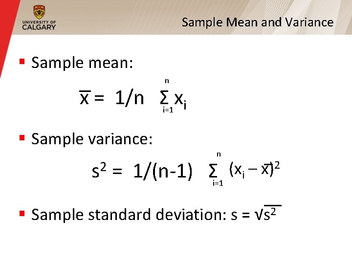
Sample Mean and Variance § Sample mean: n x = 1/n Σi=1 xi § Sample variance: s 2 n = 1/(n-1) Σi=1 (xi – x)2 § Sample standard deviation: s = √s 2

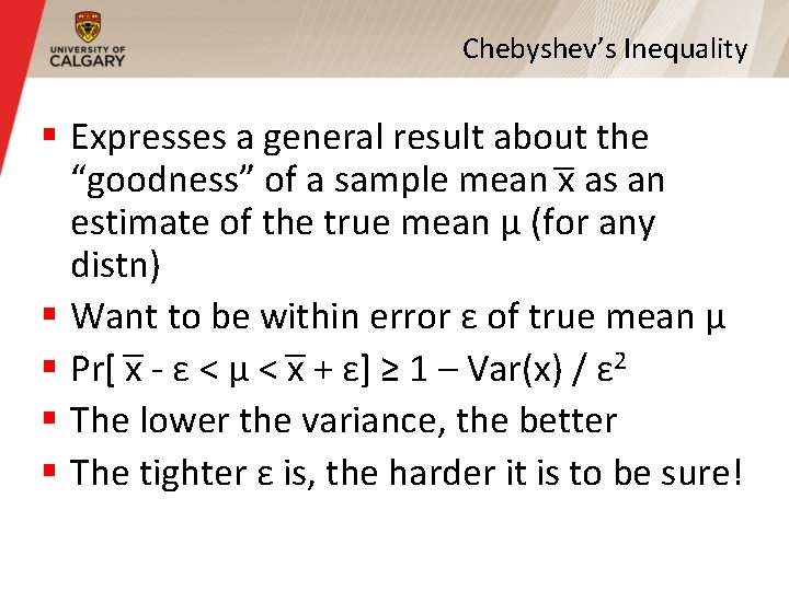
Chebyshev’s Inequality § Expresses a general result about the “goodness” of a sample mean x as an estimate of the true mean μ (for any distn) § Want to be within error ε of true mean μ § Pr[ x - ε < μ < x + ε] ≥ 1 – Var(x) / ε 2 § The lower the variance, the better § The tighter ε is, the harder it is to be sure!

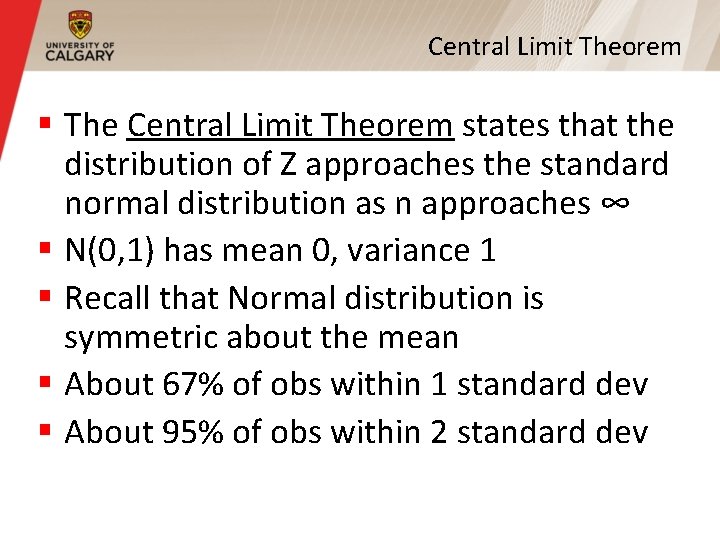
Central Limit Theorem § The Central Limit Theorem states that the distribution of Z approaches the standard normal distribution as n approaches ∞ § N(0, 1) has mean 0, variance 1 § Recall that Normal distribution is symmetric about the mean § About 67% of obs within 1 standard dev § About 95% of obs within 2 standard dev

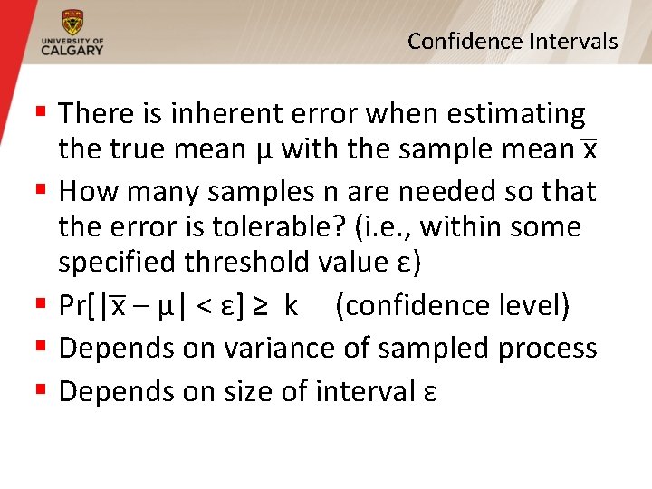
Confidence Intervals § There is inherent error when estimating the true mean μ with the sample mean x § How many samples n are needed so that the error is tolerable? (i. e. , within some specified threshold value ε) § Pr[|x – μ| < ε] ≥ k (confidence level) § Depends on variance of sampled process § Depends on size of interval ε

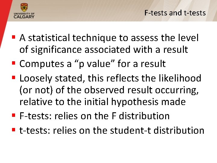
F-tests and t-tests § A statistical technique to assess the level of significance associated with a result § Computes a “p value” for a result § Loosely stated, this reflects the likelihood (or not) of the observed result occurring, relative to the initial hypothesis made § F-tests: relies on the F distribution § t-tests: relies on the student-t distribution

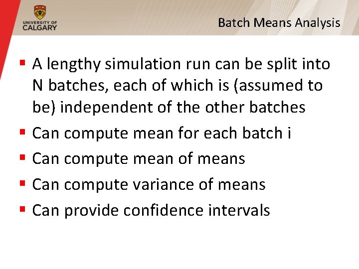
Batch Means Analysis § A lengthy simulation run can be split into N batches, each of which is (assumed to be) independent of the other batches § Can compute mean for each batch i § Can compute mean of means § Can compute variance of means § Can provide confidence intervals

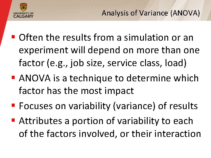
Analysis of Variance (ANOVA) § Often the results from a simulation or an experiment will depend on more than one factor (e. g. , job size, service class, load) § ANOVA is a technique to determine which factor has the most impact § Focuses on variability (variance) of results § Attributes a portion of variability to each of the factors involved, or their interaction

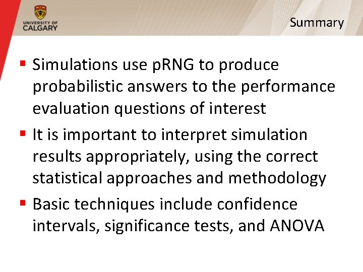
Summary § Simulations use p. RNG to produce probabilistic answers to the performance evaluation questions of interest § It is important to interpret simulation results appropriately, using the correct statistical approaches and methodology § Basic techniques include confidence intervals, significance tests, and ANOVA