CPSC 531 System Modeling and Simulation Carey Williamson

CPSC 531: System Modeling and Simulation Carey Williamson Department of Computer Science University of Calgary Fall 2017

Motivational Quote “If you can’t measure it, you can’t improve it. ” - Peter Drucker 2

(Slightly Revised) Motivational Quote model “If you can’t measure it, you can’t improve it. ” - Peter Drucker 3

Simulation Input Analysis § Input models are the driving force for many simulations § Quality of the output depends on the quality of inputs § There are four main steps for input model development: Collect data from the real system 2. Identify a suitable probability distribution to represent the input process 3. Choose parameters for the distribution 4. Evaluate the goodness-of-fit for the chosen distribution and parameters 1. 4

Data Collection § Data collection is one of the biggest simulation tasks § Beware of GIGO: Garbage-In-Garbage-Out § Suggestions to facilitate data collection: — Analyze the data as it is being collected: check adequacy — Combine homogeneous data sets (e. g. successive time periods, or the same time period on successive days) — Be aware of inadvertent data censoring: quantities that are only partially observed versus observed in their entirety; gaps; outliers; risk of leaving out long processing times — Collect input data, not performance data (i. e. , output) 5

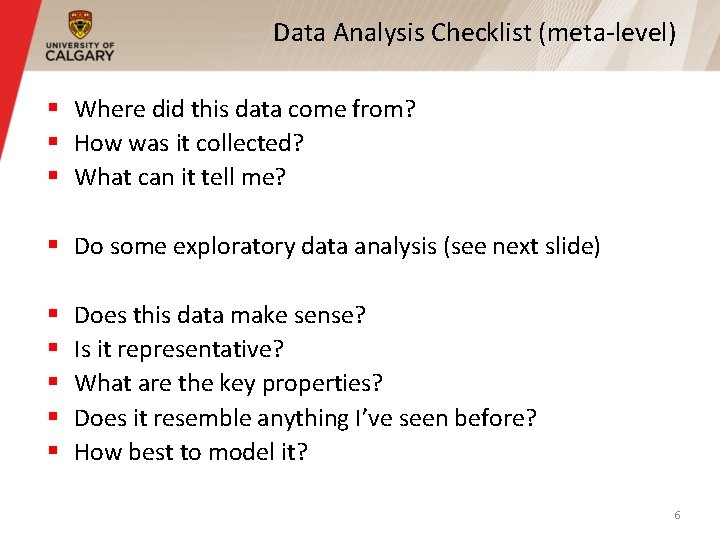
Data Analysis Checklist (meta-level) § Where did this data come from? § How was it collected? § What can it tell me? § Do some exploratory data analysis (see next slide) § § § Does this data make sense? Is it representative? What are the key properties? Does it resemble anything I’ve seen before? How best to model it? 6

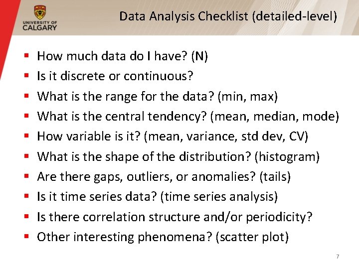
Data Analysis Checklist (detailed-level) § § § § § How much data do I have? (N) Is it discrete or continuous? What is the range for the data? (min, max) What is the central tendency? (mean, median, mode) How variable is it? (mean, variance, std dev, CV) What is the shape of the distribution? (histogram) Are there gaps, outliers, or anomalies? (tails) Is it time series data? (time series analysis) Is there correlation structure and/or periodicity? Other interesting phenomena? (scatter plot) 7

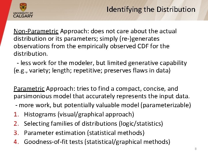
Identifying the Distribution Non-Parametric Approach: does not care about the actual distribution or its parameters; simply (re-)generates observations from the empirically observed CDF for the distribution. - less work for the modeler, but limited generative capability (e. g. , variety; length; repetitive; preserves flaws in data) Parametric Approach: tries to find a compact, concise, and parsimonious model that accurately represents the input data. - more work, but potentially valuable model (parameterizable) 1. Histograms (visual/graphical approach) 2. Selecting families of distributions (logic/statistics) 3. Parameter estimation (statistical methods) 4. Goodness-of-fit tests (statistical/graphical methods) 8

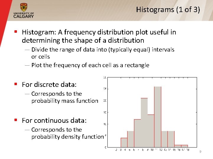
Histograms (1 of 3) § Histogram: A frequency distribution plot useful in determining the shape of a distribution — Divide the range of data into (typically equal) intervals or cells — Plot the frequency of each cell as a rectangle § For discrete data: — Corresponds to the probability mass function § For continuous data: — Corresponds to the probability density function 9

Histograms (2 of 3) § 10

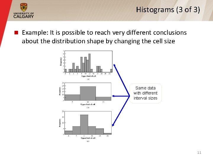
Histograms (3 of 3) Example: It is possible to reach very different conclusions about the distribution shape by changing the cell size Same data with different interval sizes 11

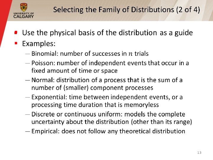
Selecting the Family of Distributions (1 of 4) § A family of distributions is selected based on: — The context of the input variable — Shape of the histogram § Frequently encountered distributions: — Easier to analyze: Exponential, Geometric, Poisson — Moderate to analyze: Normal, Log-Normal, Uniform — Harder to analyze: Beta, Gamma, Pareto, Weibull, Zipf 12

Selecting the Family of Distributions (2 of 4) § 13

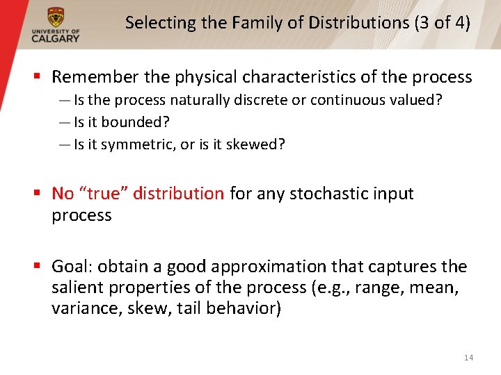
Selecting the Family of Distributions (3 of 4) § Remember the physical characteristics of the process — Is the process naturally discrete or continuous valued? — Is it bounded? — Is it symmetric, or is it skewed? § No “true” distribution for any stochastic input process § Goal: obtain a good approximation that captures the salient properties of the process (e. g. , range, mean, variance, skew, tail behavior) 14

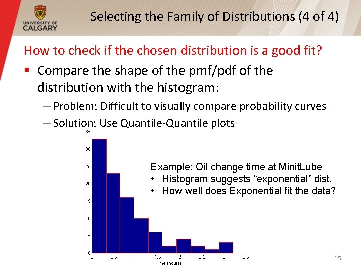
Selecting the Family of Distributions (4 of 4) How to check if the chosen distribution is a good fit? § Compare the shape of the pmf/pdf of the distribution with the histogram: — Problem: Difficult to visually compare probability curves — Solution: Use Quantile-Quantile plots Example: Oil change time at Minit. Lube • Histogram suggests “exponential” dist. • How well does Exponential fit the data? 15

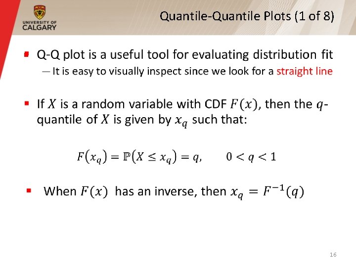
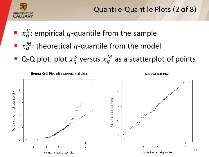
Quantile-Quantile Plots (1 of 8) § 16

Quantile-Quantile Plots (2 of 8) § 17

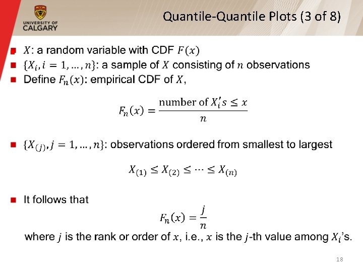
Quantile-Quantile Plots (3 of 8) § 18

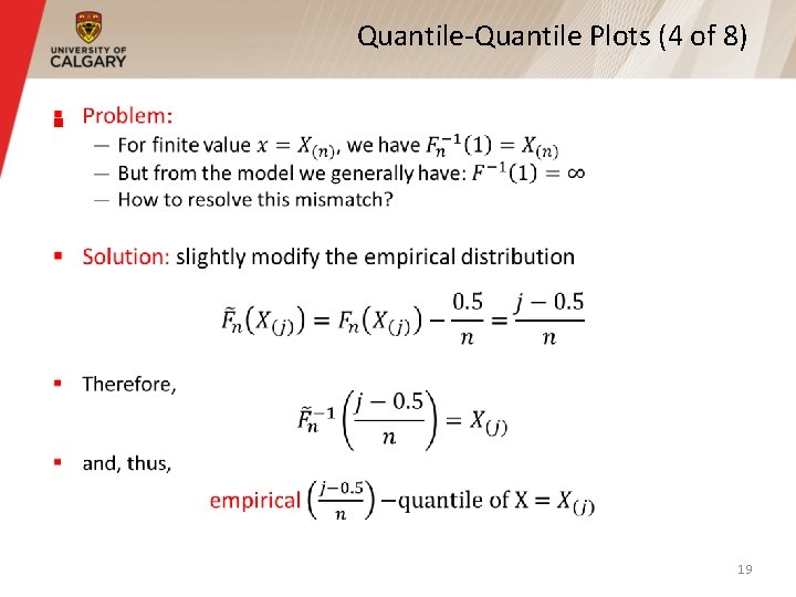
Quantile-Quantile Plots (4 of 8) § 19

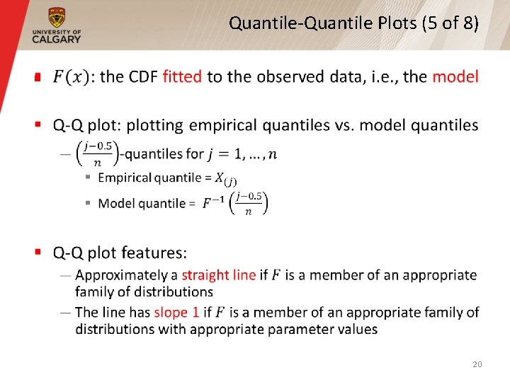
Quantile-Quantile Plots (5 of 8) § 20

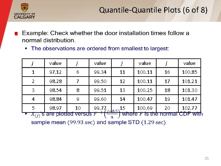
Quantile-Quantile Plots (6 of 8) § value 1 97. 12 6 99. 34 11 100. 11 16 100. 85 2 98. 28 7 99. 50 12 100. 11 17 101. 21 3 98. 54 8 99. 51 13 100. 25 18 101. 30 4 98. 84 9 99. 60 14 100. 47 19 101. 47 5 98. 97 10 99. 77 15 100. 69 20 102. 77 21

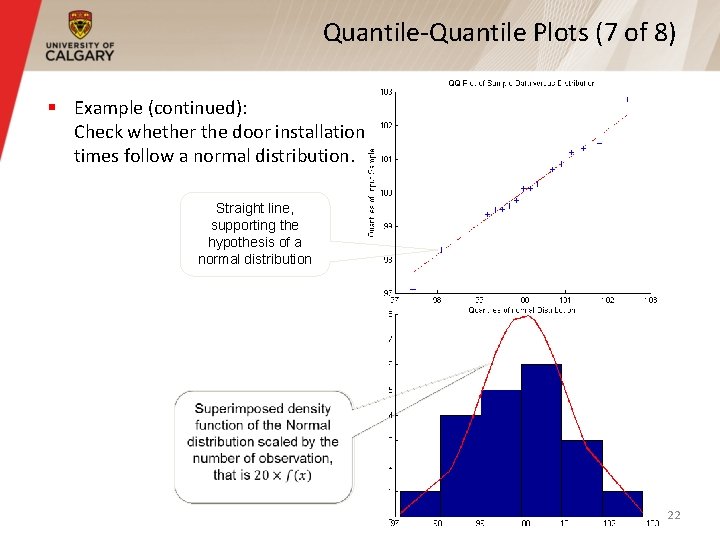
Quantile-Quantile Plots (7 of 8) § Example (continued): Check whether the door installation times follow a normal distribution. Straight line, supporting the hypothesis of a normal distribution 22

Quantile-Quantile Plots (8 of 8) § Consider the following while evaluating the linearity of a Q-Q plot: — The observed values never fall exactly on a straight line — Variation of the extremes is higher than the middle. — Linearity of the points in the middle of the plot (the main body of the distribution) is more important. 23

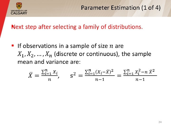
Parameter Estimation (1 of 4) § 24

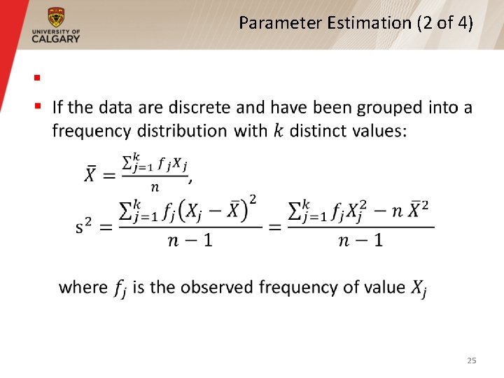
Parameter Estimation (2 of 4) § 25

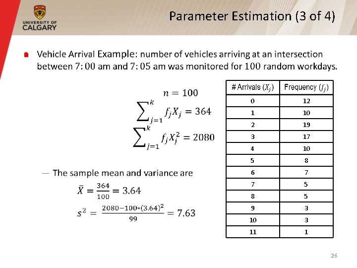
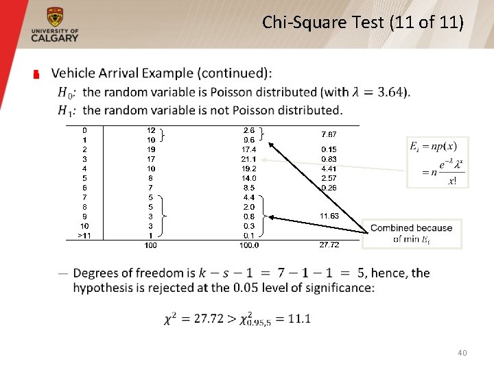
Parameter Estimation (3 of 4) § 0 12 1 10 2 19 3 17 4 10 5 8 6 7 7 5 8 5 9 3 10 3 11 1 26

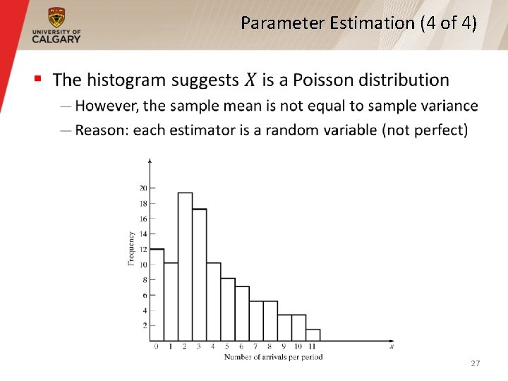
Parameter Estimation (4 of 4) § 27

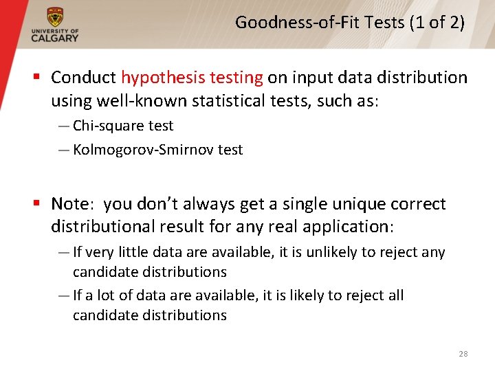
Goodness-of-Fit Tests (1 of 2) § Conduct hypothesis testing on input data distribution using well-known statistical tests, such as: — Chi-square test — Kolmogorov-Smirnov test § Note: you don’t always get a single unique correct distributional result for any real application: — If very little data are available, it is unlikely to reject any candidate distributions — If a lot of data are available, it is likely to reject all candidate distributions 28

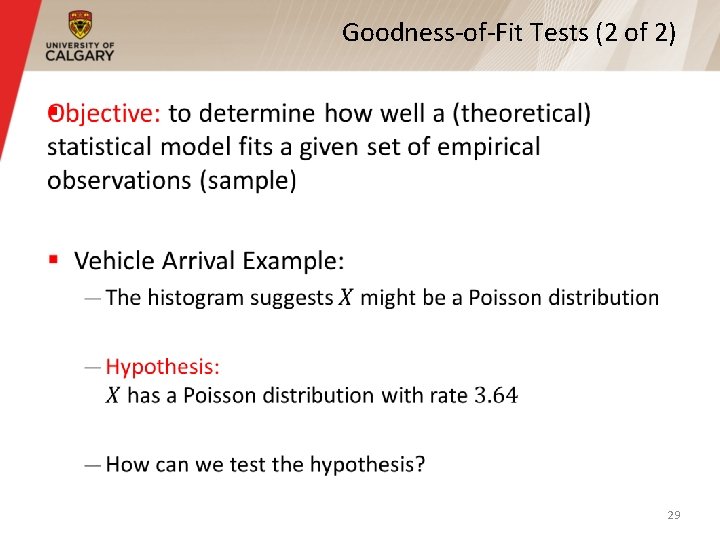
Goodness-of-Fit Tests (2 of 2) § 29

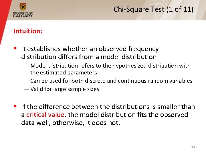
Chi-Square Test (1 of 11) Intuition: § It establishes whether an observed frequency distribution differs from a model distribution — Model distribution refers to the hypothesized distribution with the estimated parameters — Can be used for both discrete and continuous random variables — Valid for large sample sizes § If the difference between the distributions is smaller than a critical value, the model distribution fits the observed data well, otherwise, it does not. 30

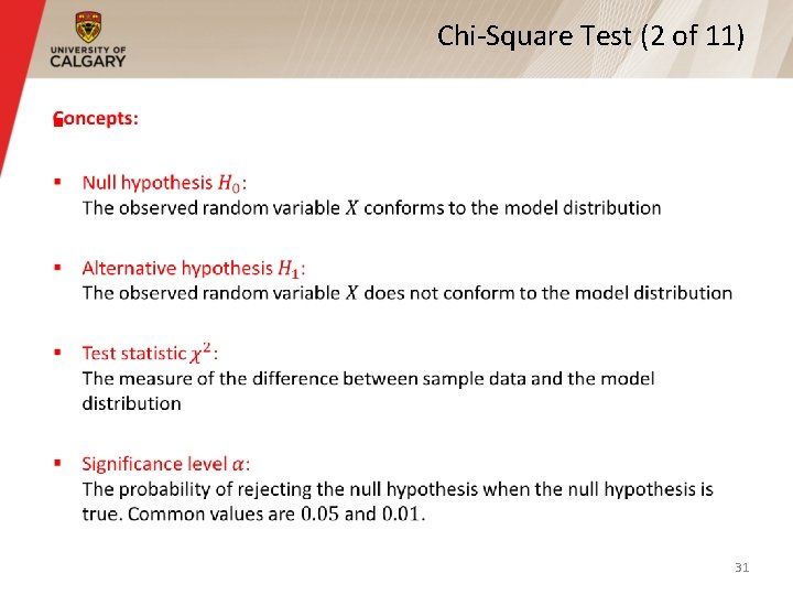
Chi-Square Test (2 of 11) § 31

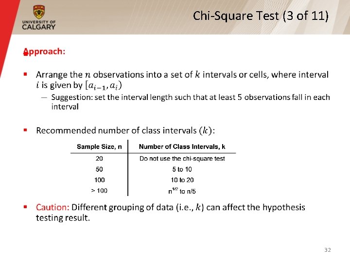
Chi-Square Test (3 of 11) § 32

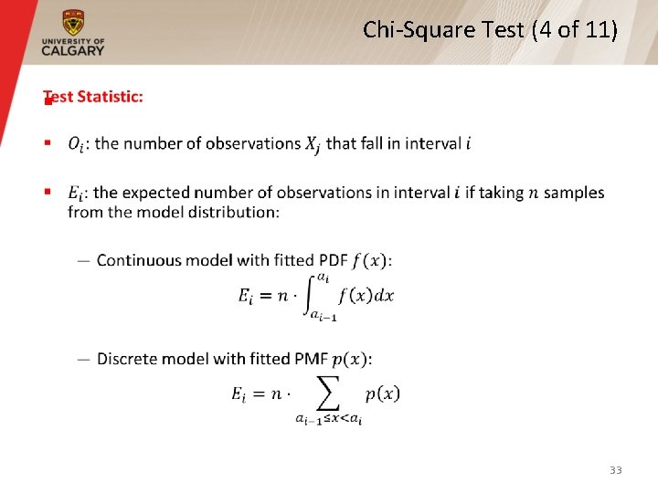
Chi-Square Test (4 of 11) § 33

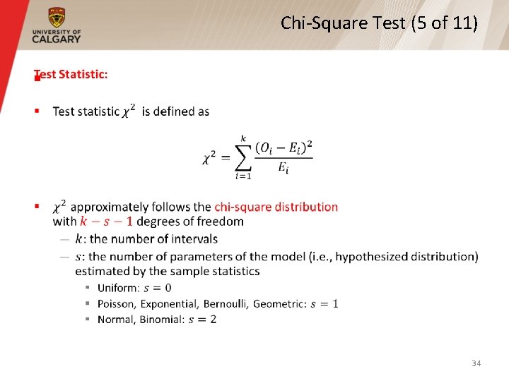
Chi-Square Test (5 of 11) § 34

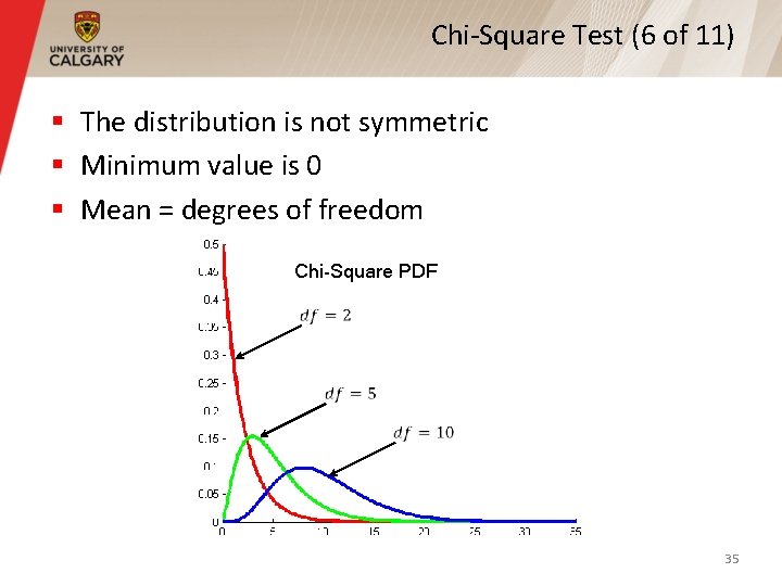
Chi-Square Test (6 of 11) § The distribution is not symmetric § Minimum value is 0 § Mean = degrees of freedom Chi-Square PDF 35

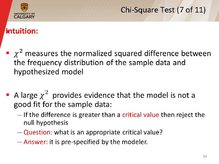
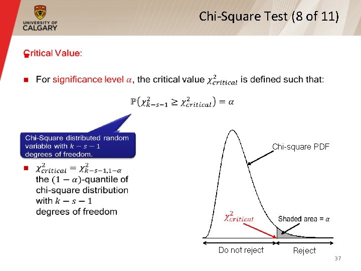
Chi-Square Test (7 of 11) § 36

Chi-Square Test (8 of 11) § Chi-square PDF Do not reject Reject 37

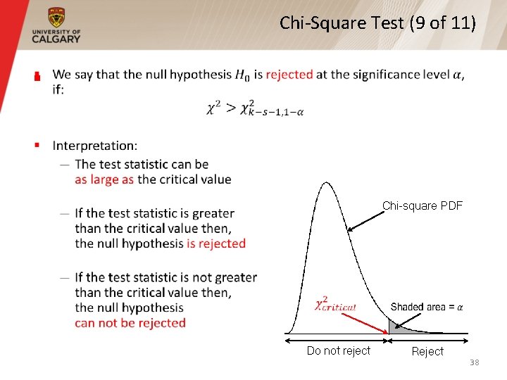
Chi-Square Test (9 of 11) § Chi-square PDF Do not reject Reject 38

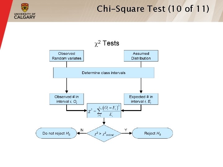
Chi-Square Test (10 of 11)

Chi-Square Test (11 of 11) § 40

Kolmogorov-Smirnov Test § Intuition: — Formalizes the idea behind examining a Q-Q plot — The test compares the CDF of the hypothesized distribution with the empirical CDF of the sample observations based on the maximum distance between two cumulative distribution functions. § A more powerful test that is particularly useful when: — Sample sizes are small — No parameters have been estimated from the data 41

Selecting Model without Data (1 of 2) § If data is not available, some possible sources to obtain information about the process are: — Engineering data: often product or process has performance ratings provided by the manufacturer or company that specify time or production standards — Expert option: people who are experienced with the process or similar processes, often, they can provide optimistic, pessimistic and mostlikely times, and they may know the variability as well — Physical or conventional limitations: physical limits on performance, limits or bounds that narrow the range of the input process — The nature of the process § The uniform, triangular, and beta distributions are often used as input models. 42

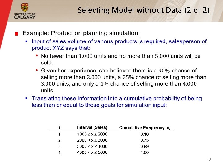
Selecting Model without Data (2 of 2) § 43

Multivariate and Time-Series Models § So far, we have considered: — Single variate models for independent input parameters § To model correlation among input parameters — Multivariate models — Time-series models 44