CPSC 531 System Modeling and Simulation Carey Williamson

CPSC 531: System Modeling and Simulation Carey Williamson Department of Computer Science University of Calgary Fall 2017

Quote of the Day § “The generation of random numbers is too important to be left to chance” - Steve Park (R. Coveyou) § Main messages: — Need great rigour in design and use of (P)RNG — Need great care in RVG process as well (avoid GIGO!) — Verification and validation apply here as well! 2

Outline § Common Discrete Distributions § Common Continuous Distributions § RVG Testing — Uniformity — Independence — Mean and variance — Central tendency: mean, median, mode — Extreme values: min and max — Visual appearance: pdf and CDF — Autocorrelation properties 3

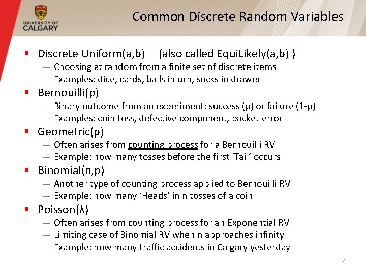
Common Discrete Random Variables § Discrete Uniform(a, b) (also called Equi. Likely(a, b) ) — Choosing at random from a finite set of discrete items — Examples: dice, cards, balls in urn, socks in drawer § Bernouilli(p) — Binary outcome from an experiment: success (p) or failure (1 -p) — Examples: coin toss, defective component, packet error § Geometric(p) — Often arises from counting process for a Bernouilli RV — Example: how many tosses before the first ‘Tail’ occurs § Binomial(n, p) — Another type of counting process applied to Bernouilli RV — Example: how many ‘Heads’ in n tosses of a coin § Poisson(λ) — Often arises from counting process for an Exponential RV — Limiting case of Binomial RV when n approaches infinity — Example: how many traffic accidents in Calgary yesterday 4

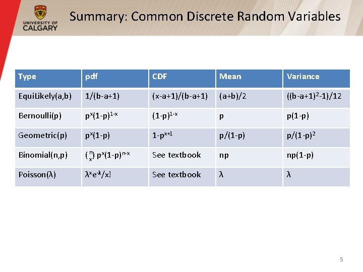
Summary: Common Discrete Random Variables Type pdf CDF Mean Variance Equi. Likely(a, b) 1/(b-a+1) (x-a+1)/(b-a+1) (a+b)/2 ((b-a+1)2 -1)/12 Bernoulli(p) px(1 -p)1 -x p p(1 -p) Geometric(p) px(1 -p) 1 -px+1 p/(1 -p)2 Binomial(n, p) ( nx) px(1 -p)n-x See textbook np np(1 -p) Poisson(λ) λxe-λ/x! See textbook λ λ 5

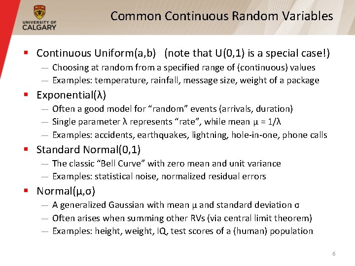
Common Continuous Random Variables § Continuous Uniform(a, b) (note that U(0, 1) is a special case!) — Choosing at random from a specified range of (continuous) values — Examples: temperature, rainfall, message size, weight of a package § Exponential(λ) — Often a good model for “random” events (arrivals, duration) — Single parameter λ represents “rate”, while mean μ = 1/λ — Examples: accidents, earthquakes, lightning, hole-in-one, phone calls § Standard Normal(0, 1) — The classic “Bell Curve” with zero mean and unit variance — Examples: statistical noise, normalized residual errors § Normal(μ, σ) — A generalized Gaussian with mean μ and standard deviation σ — Often arises when summing other RVs (via central limit theorem) — Examples: height, weight, IQ, test scores of a (human) population 6

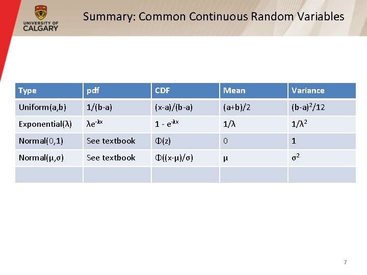
Summary: Common Continuous Random Variables Type pdf CDF Mean Variance Uniform(a, b) 1/(b-a) (x-a)/(b-a) (a+b)/2 (b-a)2/12 Exponential(λ) λe-λx 1 - e-λx 1/λ 2 Normal(0, 1) See textbook Φ(z) 0 1 Normal(μ, σ) See textbook Φ((x-μ)/σ) μ σ2 7

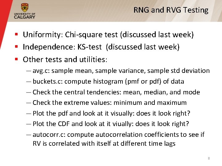
RNG and RVG Testing § Uniformity: Chi-square test (discussed last week) § Independence: KS-test (discussed last week) § Other tests and utilities: — avg. c: sample mean, sample variance, sample std deviation — buckets. c: compute histogram (pmf or pdf) of data — Check the central tendencies: mean, median, and mode — Check the extreme values: minimum and maximum — Plot the pdf and look at it visually: does it look right? — Plot the CDF and look at it viually: does it look right? — autocorr. c: compute autocorrelation coefficients to see if RV is correlated with itself at different time lags 8