Correlation and Regression 17 2 Product Moment Correlation

Correlation and Regression

17 -2 Product Moment Correlation n The product moment correlation, r, summarizes the strength of association between two metric (interval or ratio scaled) variables, say X and Y. It is an index used to determine whether a linear or straight-line relationship exists between X and Y. As it was originally proposed by Karl Pearson, it is also known as the Pearson correlation coefficient. It is also referred to as simple correlation, bivariate correlation, or merely the correlation coefficient.

17 -3 Product Moment Correlation n n r varies between -1. 0 and +1. 0. The correlation coefficient between two variables will be the same regardless of their underlying units of measurement.

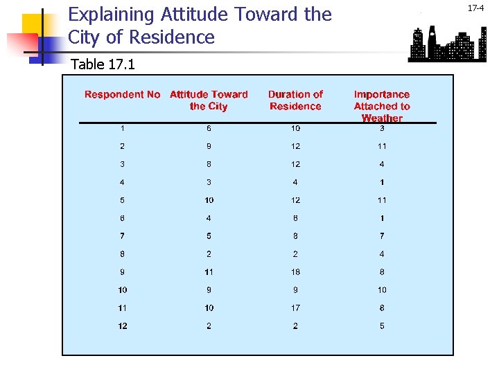
Explaining Attitude Toward the City of Residence Table 17. 1 17 -4

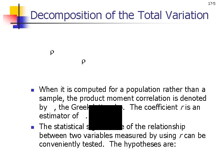
17 -5 Decomposition of the Total Variation n n When it is computed for a population rather than a sample, the product moment correlation is denoted by , the Greek letter rho. The coefficient r is an estimator of. The statistical significance of the relationship between two variables measured by using r can be conveniently tested. The hypotheses are:

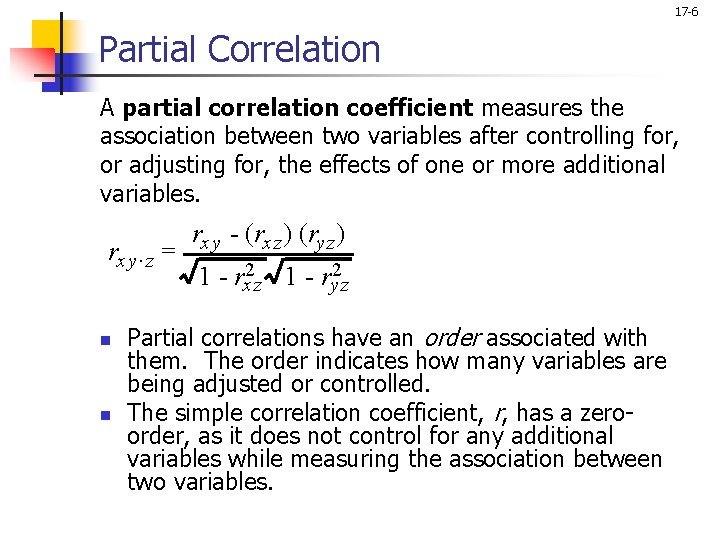
17 -6 Partial Correlation A partial correlation coefficient measures the association between two variables after controlling for, or adjusting for, the effects of one or more additional variables. rx y. z = n n rx y - (rx z ) (ry z ) 1 - rx 2 z 1 - ry 2 z Partial correlations have an order associated with them. The order indicates how many variables are being adjusted or controlled. The simple correlation coefficient, r, has a zeroorder, as it does not control for any additional variables while measuring the association between two variables.

17 -7 Partial Correlation n The coefficient rxy. z is a first-order partial correlation coefficient, as it controls for the effect of one additional variable, Z. A second-order partial correlation coefficient controls for the effects of two variables, a third-order for the effects of three variables, and so on. The special case when a partial correlation is larger than its respective zero-order correlation involves a suppressor effect.

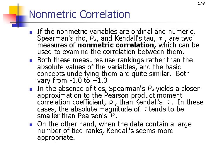
17 -8 Nonmetric Correlation n n If the nonmetric variables are ordinal and numeric, Spearman's rho, , and Kendall's tau, , are two measures of nonmetric correlation, which can be used to examine the correlation between them. Both these measures use rankings rather than the absolute values of the variables, and the basic concepts underlying them are quite similar. Both vary from -1. 0 to +1. 0 In the absence of ties, Spearman's yields a closer approximation to the Pearson product moment correlation coefficient, , than Kendall's. In these cases, the absolute magnitude of tends to be smaller than Pearson's. On the other hand, when the data contain a large number of tied ranks, Kendall's seems more appropriate.

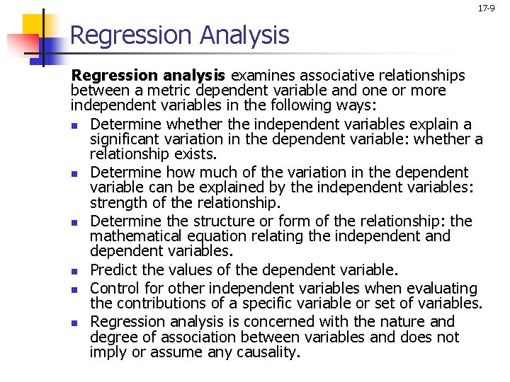
17 -9 Regression Analysis Regression analysis examines associative relationships between a metric dependent variable and one or more independent variables in the following ways: n Determine whether the independent variables explain a significant variation in the dependent variable: whether a relationship exists. n Determine how much of the variation in the dependent variable can be explained by the independent variables: strength of the relationship. n Determine the structure or form of the relationship: the mathematical equation relating the independent and dependent variables. n Predict the values of the dependent variable. n Control for other independent variables when evaluating the contributions of a specific variable or set of variables. n Regression analysis is concerned with the nature and degree of association between variables and does not imply or assume any causality.

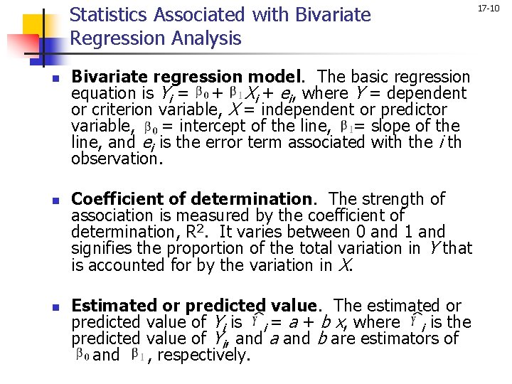
Statistics Associated with Bivariate Regression Analysis n n n Bivariate regression model. The basic regression equation is Yi = + Xi + ei, where Y = dependent or criterion variable, X = independent or predictor variable, = intercept of the line, = slope of the line, and ei is the error term associated with the i th observation. Coefficient of determination. The strength of association is measured by the coefficient of determination, R 2. It varies between 0 and 1 and signifies the proportion of the total variation in Y that is accounted for by the variation in X. Estimated or predicted value. The estimated or predicted value of Yi is i = a + b x, where i is the predicted value of Yi, and a and b are estimators of and , respectively. 17 -10

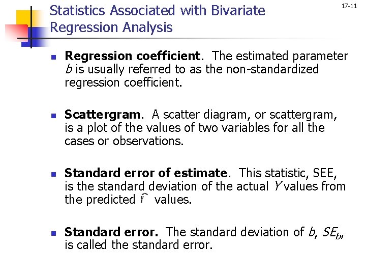
Statistics Associated with Bivariate Regression Analysis n n 17 -11 Regression coefficient. The estimated parameter b is usually referred to as the non-standardized regression coefficient. Scattergram. A scatter diagram, or scattergram, is a plot of the values of two variables for all the cases or observations. Standard error of estimate. This statistic, SEE, is the standard deviation of the actual Y values from the predicted values. Standard error. The standard deviation of b, SEb, is called the standard error.

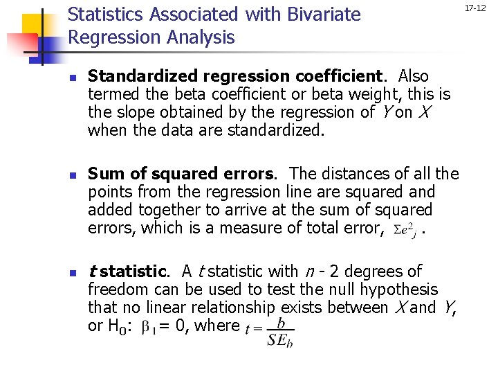
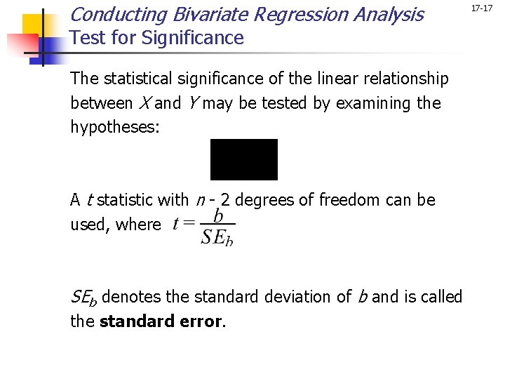
Statistics Associated with Bivariate Regression Analysis n n n Standardized regression coefficient. Also termed the beta coefficient or beta weight, this is the slope obtained by the regression of Y on X when the data are standardized. Sum of squared errors. The distances of all the points from the regression line are squared and added together to arrive at the sum of squared errors, which is a measure of total error, . t statistic. A t statistic with n - 2 degrees of freedom can be used to test the null hypothesis that no linear relationship exists between X and Y, or H 0: = 0, where 17 -12

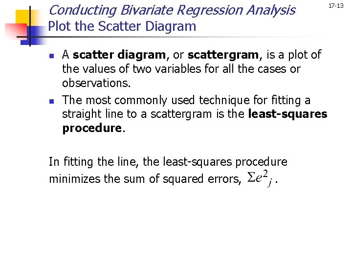
Conducting Bivariate Regression Analysis Plot the Scatter Diagram n n A scatter diagram, or scattergram, is a plot of the values of two variables for all the cases or observations. The most commonly used technique for fitting a straight line to a scattergram is the least-squares procedure. In fitting the line, the least-squares procedure minimizes the sum of squared errors, . 17 -13

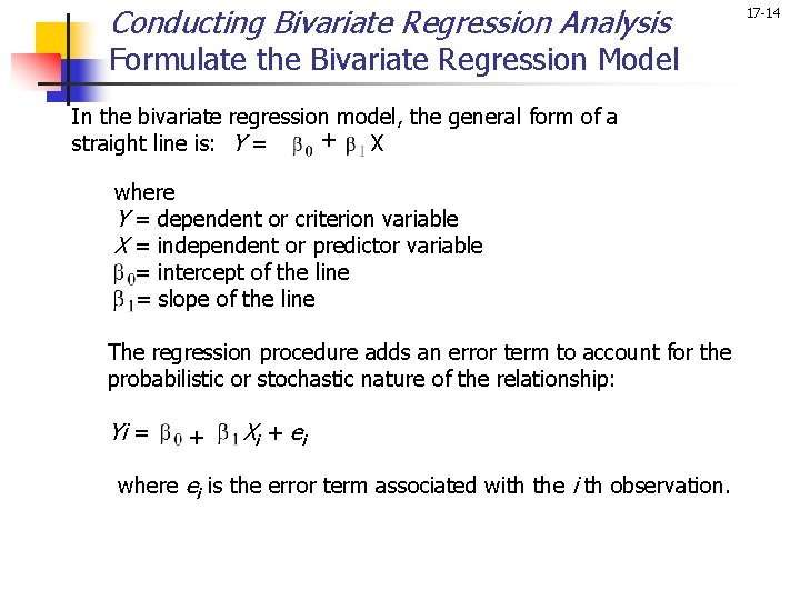
Conducting Bivariate Regression Analysis Formulate the Bivariate Regression Model In the bivariate regression model, the general form of a + straight line is: Y = X where Y = dependent or criterion variable X = independent or predictor variable = intercept of the line = slope of the line The regression procedure adds an error term to account for the probabilistic or stochastic nature of the relationship: Yi = + X i + ei where ei is the error term associated with the i th observation. 17 -14

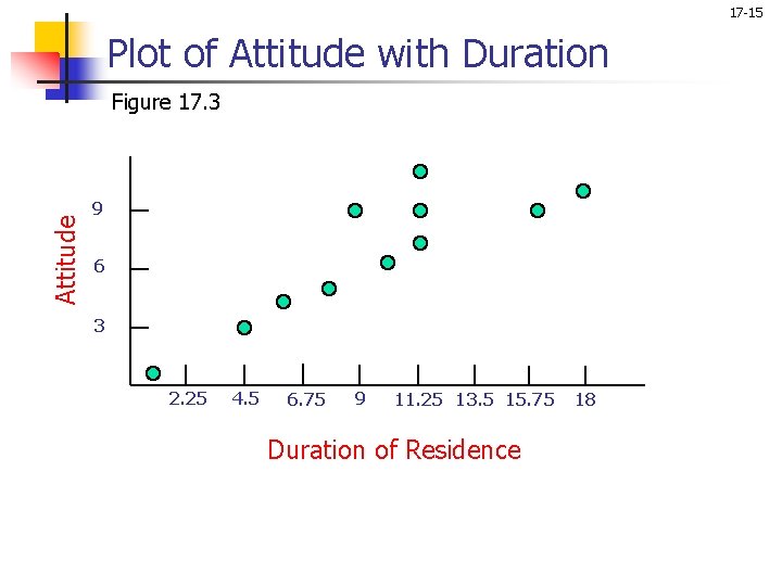
17 -15 Plot of Attitude with Duration Attitude Figure 17. 3 9 6 3 2. 25 4. 5 6. 75 9 11. 25 13. 5 15. 75 Duration of Residence 18

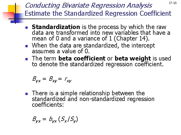
Conducting Bivariate Regression Analysis 17 -16 Estimate the Standardized Regression Coefficient n n n Standardization is the process by which the raw data are transformed into new variables that have a mean of 0 and a variance of 1 (Chapter 14). When the data are standardized, the intercept assumes a value of 0. The term beta coefficient or beta weight is used to denote the standardized regression coefficient. Byx = Bxy = rxy n There is a simple relationship between the standardized and non-standardized regression coefficients: Byx = byx (Sx /Sy)

Conducting Bivariate Regression Analysis Test for Significance The statistical significance of the linear relationship between X and Y may be tested by examining the hypotheses: A t statistic with n - 2 degrees of freedom can be used, where SEb denotes the standard deviation of b and is called the standard error. 17 -17

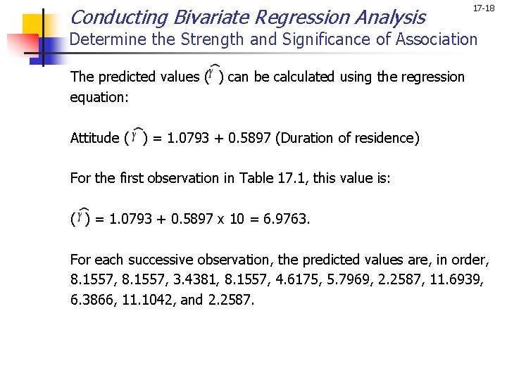
Conducting Bivariate Regression Analysis 17 -18 Determine the Strength and Significance of Association The predicted values ( ) can be calculated using the regression equation: Attitude ( ) = 1. 0793 + 0. 5897 (Duration of residence) For the first observation in Table 17. 1, this value is: ( ) = 1. 0793 + 0. 5897 x 10 = 6. 9763. For each successive observation, the predicted values are, in order, 8. 1557, 3. 4381, 8. 1557, 4. 6175, 5. 7969, 2. 2587, 11. 6939, 6. 3866, 11. 1042, and 2. 2587.

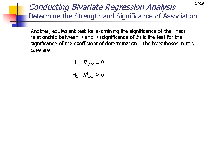
Conducting Bivariate Regression Analysis 17 -19 Determine the Strength and Significance of Association Another, equivalent test for examining the significance of the linear relationship between X and Y (significance of b) is the test for the significance of the coefficient of determination. The hypotheses in this case are: H 0: R 2 pop = 0 H 1: R 2 pop > 0

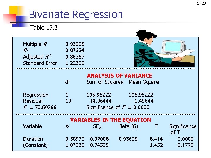
17 -20 Bivariate Regression Table 17. 2 Multiple R R 2 Adjusted R 2 Standard Error 0. 93608 0. 87624 0. 86387 1. 22329 df Regression Residual F = 70. 80266 1 10 ANALYSIS OF VARIANCE Sum of Squares Mean Square 105. 95222 14. 96444 1. 49644 Significance of F = 0. 0000 Variable VARIABLES IN THE EQUATION b SEb Beta (ß) T Duration (Constant) 0. 58972 1. 07932 0. 07008 0. 74335 0. 93608 8. 414 1. 452 Significance of T 0. 0000 0. 1772

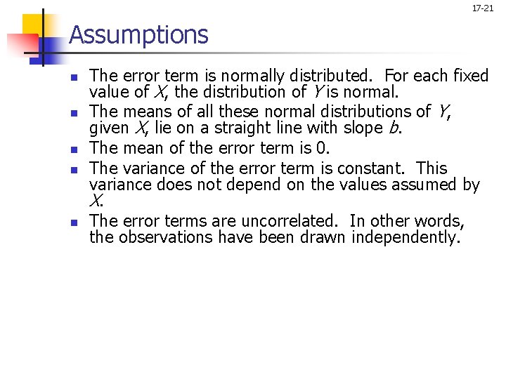
17 -21 Assumptions n n n The error term is normally distributed. For each fixed value of X, the distribution of Y is normal. The means of all these normal distributions of Y, given X, lie on a straight line with slope b. The mean of the error term is 0. The variance of the error term is constant. This variance does not depend on the values assumed by X. The error terms are uncorrelated. In other words, the observations have been drawn independently.

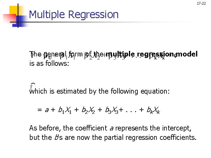
17 -22 Multiple Regression The general form of the multiple regressionemodel is as follows: which is estimated by the following equation: = a + b 1 X 1 + b 2 X 2 + b 3 X 3 +. . . + b k. X k As before, the coefficient a represents the intercept, but the b's are now the partial regression coefficients.

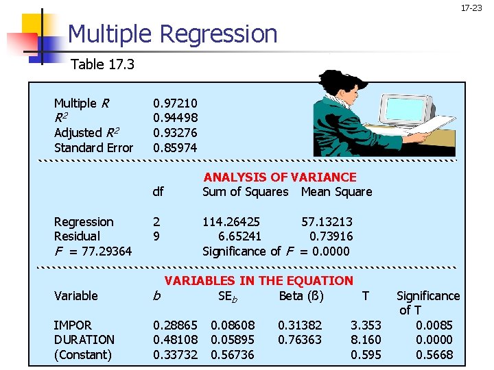
17 -23 Multiple Regression Table 17. 3 Multiple R R 2 Adjusted R 2 Standard Error 0. 97210 0. 94498 0. 93276 0. 85974 df Regression Residual F = 77. 29364 2 9 ANALYSIS OF VARIANCE Sum of Squares Mean Square 114. 26425 57. 13213 6. 65241 0. 73916 Significance of F = 0. 0000 Variable VARIABLES IN THE EQUATION b SEb Beta (ß) T IMPOR DURATION (Constant) 0. 28865 0. 48108 0. 33732 0. 08608 0. 05895 0. 56736 0. 31382 0. 76363 3. 353 8. 160 0. 595 Significance of T 0. 0085 0. 0000 0. 5668

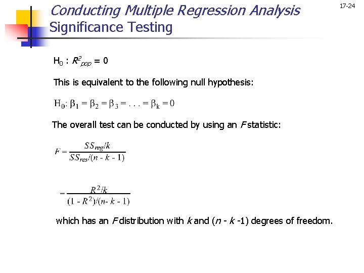
Conducting Multiple Regression Analysis Significance Testing H 0 : R 2 pop = 0 This is equivalent to the following null hypothesis: The overall test can be conducted by using an F statistic: which has an F distribution with k and (n - k -1) degrees of freedom. 17 -24

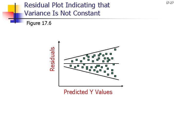
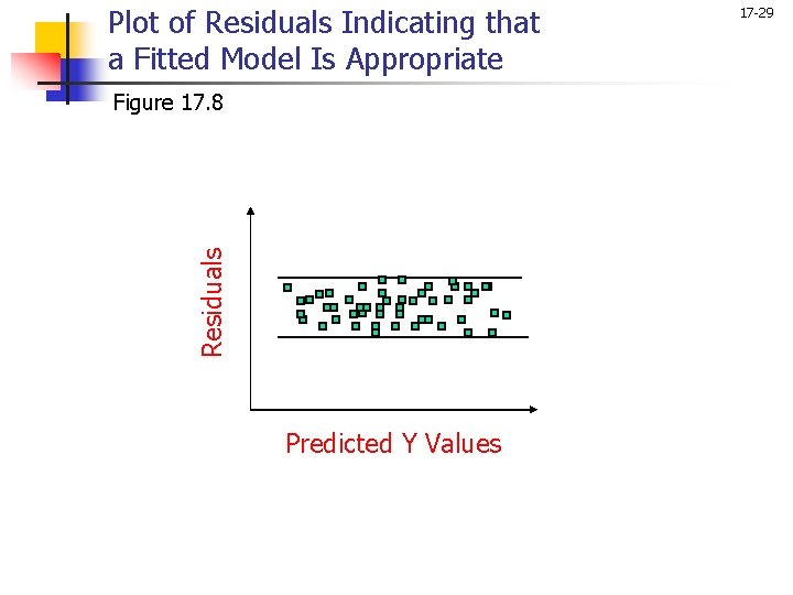
Conducting Multiple Regression Analysis 17 -25 Examination of Residuals n n A residual is the difference between the observed value of Yi and the value predicted by the regression equation Yi. Scattergrams of the residuals, in which the residuals are plotted against the predicted values, i, time, or predictor variables, provide useful insights in examining the appropriateness of the underlying assumptions and regression model fit. The assumption of a normally distributed error term can be examined by constructing a histogram of the residuals. The assumption of constant variance of the error term can be examined by plotting the residuals against the predicted values of the dependent variable, i.

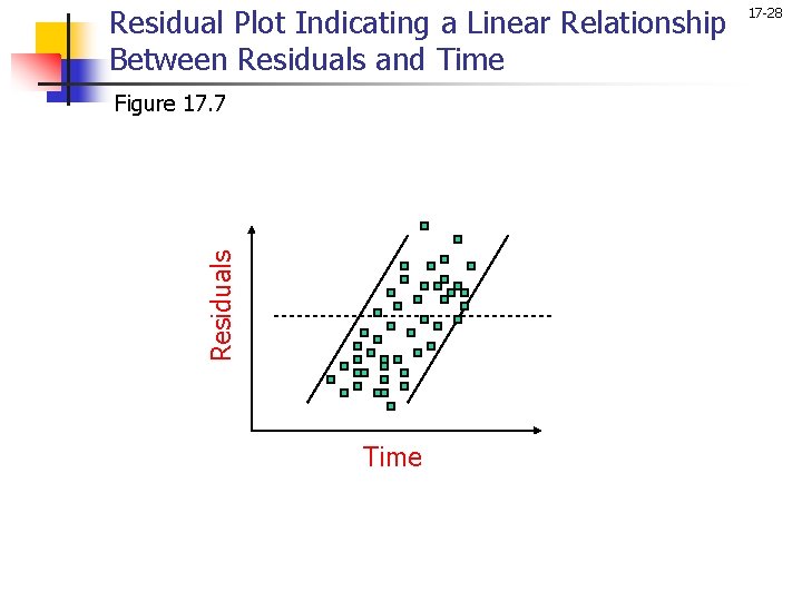
Conducting Multiple Regression Analysis 17 -26 Examination of Residuals n n A plot of residuals against time, or the sequence of observations, will throw some light on the assumption that the error terms are uncorrelated. Plotting the residuals against the independent variables provides evidence of the appropriateness or inappropriateness of using a linear model. Again, the plot should result in a random pattern. To examine whether any additional variables should be included in the regression equation, one could run a regression of the residuals on the proposed variables. If an examination of the residuals indicates that the assumptions underlying linear regression are not met, the researcher can transform the variables in an attempt to satisfy the assumptions.

Residual Plot Indicating that Variance Is Not Constant Residuals Figure 17. 6 Predicted Y Values 17 -27

Residual Plot Indicating a Linear Relationship Between Residuals and Time Residuals Figure 17. 7 Time 17 -28

Plot of Residuals Indicating that a Fitted Model Is Appropriate Residuals Figure 17. 8 Predicted Y Values 17 -29

17 -30 Multicollinearity n n Multicollinearity arises when intercorrelations among the predictors are very high. Multicollinearity can result in several problems, including: n The partial regression coefficients may not be estimated precisely. The standard errors are likely to be high. n The magnitudes as well as the signs of the partial regression coefficients may change from sample to sample. n It becomes difficult to assess the relative importance of the independent variables in explaining the variation in the dependent variable. n Predictor variables may be incorrectly included or removed in stepwise regression.

17 -31 Multicollinearity n n n A simple procedure for adjusting for multicollinearity consists of using only one of the variables in a highly correlated set of variables. Alternatively, the set of independent variables can be transformed into a new set of predictors that are mutually independent by using techniques such as principal components analysis. More specialized techniques, such as ridge regression and latent root regression, can also be used.

17 -32 SPSS Windows The CORRELATE program computes Pearson product moment correlations and partial correlations with significance levels. Univariate statistics, covariance, and cross-product deviations may also be requested. Significance levels are included in the output. To select these procedures using SPSS for Windows click: Analyze>Correlate>Bivariate … Analyze>Correlate>Partial … Scatterplots can be obtained by clicking: Graphs>Scatter …>Simple>Define REGRESSION calculates bivariate and multiple regression equations, associated statistics, and plots. It allows for an easy examination of residuals. This procedure can be run by clicking: Analyze>Regression Linear …