Correlation and Simple Linear Regression Pearsons Product Moment

Correlation and Simple Linear Regression

Pearson’s Product Moment Correlation (sample correlation r estimates population correlation r) • Measures the strength of linear association between two numeric variables X and Y. • The correlation (r) is a unit-less quantity. • -1 < r < 1 • If r < 0 then there is a negative association between X and Y, i. e. as X increases Y generally decreases • If r > 0 then there is a positive association between X and Y, i. e. as X increases Y generally increases

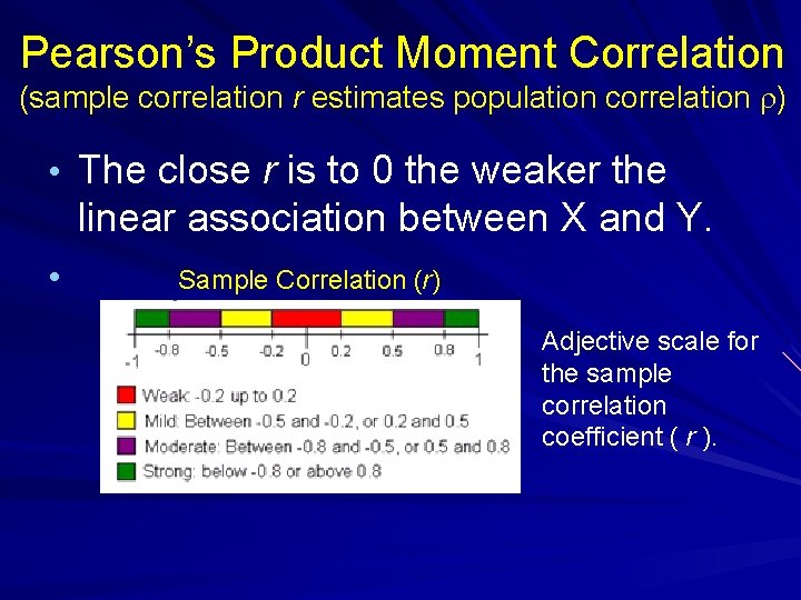
Pearson’s Product Moment Correlation (sample correlation r estimates population correlation r) • The close r is to 0 the weaker the linear association between X and Y. • Sample Correlation (r) Adjective scale for the sample correlation coefficient ( r ).

Pearson’s Product Moment Correlation ( r ) Some examples of various positive and negative correlations.

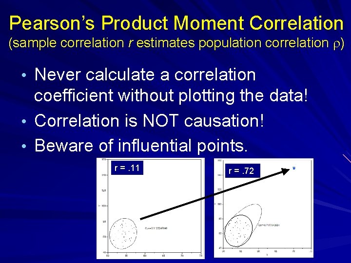
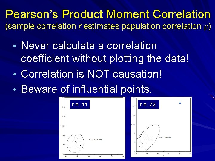
Pearson’s Product Moment Correlation (sample correlation r estimates population correlation r) • Never calculate a correlation • • coefficient without plotting the data! Correlation is NOT causation! Beware of influential points. r =. 11 r =. 72

Pearson’s Product Moment Correlation (sample correlation r estimates population correlation r) • Never calculate a correlation • • coefficient without plotting the data! Correlation is NOT causation! Beware of influential points. r =. 11 r =. 72

Pearson’s Product Moment Correlation (sample correlation r estimates population correlation r) • Beware of outliers r =. 86 r =. 66

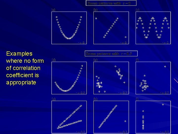
Examples where no form of correlation coefficient is appropriate

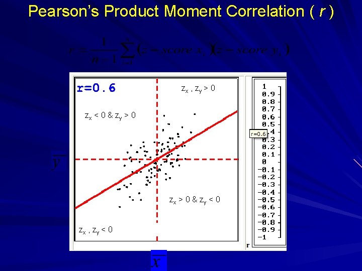
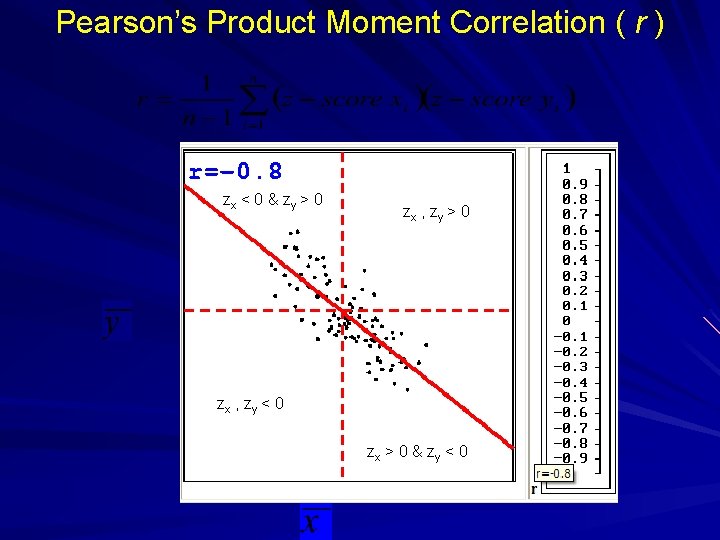
Pearson’s Product Moment Correlation ( r ) • The formula (and equivalencies)

Pearson’s Product Moment Correlation ( r ) zx , zy > 0 zx < 0 & zy > 0 zx > 0 & zy < 0 zx , zy < 0

Pearson’s Product Moment Correlation ( r ) zx < 0 & zy > 0 zx , zy < 0 zx > 0 & zy < 0

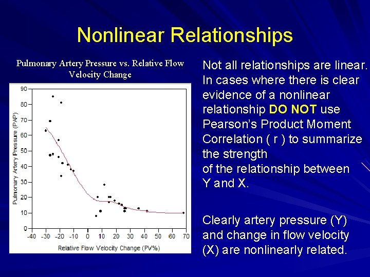
Nonlinear Relationships Pulmonary Artery Pressure vs. Relative Flow Velocity Change Not all relationships are linear. In cases where there is clear evidence of a nonlinear relationship DO NOT use Pearson’s Product Moment Correlation ( r ) to summarize the strength of the relationship between Y and X. Clearly artery pressure (Y) and change in flow velocity (X) are nonlinearly related.

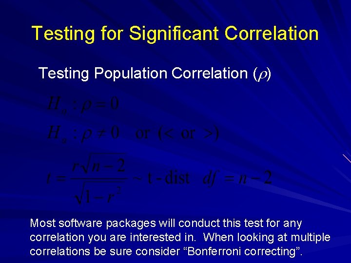
Testing for Significant Correlation Testing Population Correlation (r) Most software packages will conduct this test for any correlation you are interested in. When looking at multiple correlations be sure consider “Bonferroni correcting”.

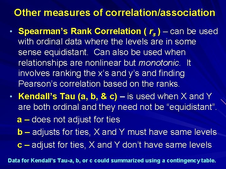
Other measures of correlation/association • Spearman’s Rank Correlation ( rs ) – can be used with ordinal data where the levels are in some sense equidistant. Can also be used when relationships are nonlinear but monotonic. It involves ranking the x’s and y’s and finding Pearson’s correlation based on the ranks. • Kendall’s Tau (a, b, & c) – is used when X and Y are both ordinal and they need not be “equidistant”. a – does not adjust for ties b – adjusts for ties, X and Y must have same levels c – adjust for ties, X and Y don’t have same levels Data for Kendall’s Tau-a, b, or c could summarized using a contingency table.

Other measures of correlation/association • Biserial Correlation – correlation when X is continuous and Y is naturally dichotomous (e. g. male/female, smoker/non-smoker) or a created (e. g. Age < 18/Age > 18). • Polyserial Correlation – correlation when X is continuous and Y is ordinal. • JMP/SPSS compute Spearman’s and Kendall’s tau however the others require specialized software.

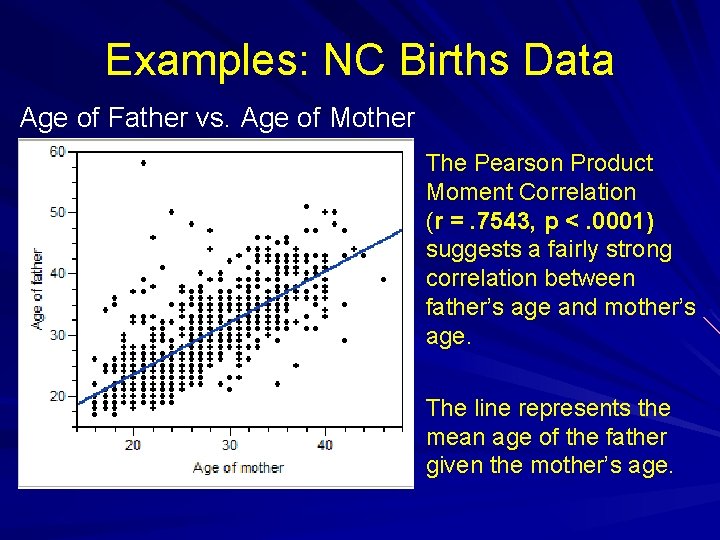
Examples: NC Births Data Age of Father vs. Age of Mother The Pearson Product Moment Correlation (r =. 7543, p <. 0001) suggests a fairly strong correlation between father’s age and mother’s age. The line represents the mean age of the father given the mother’s age.

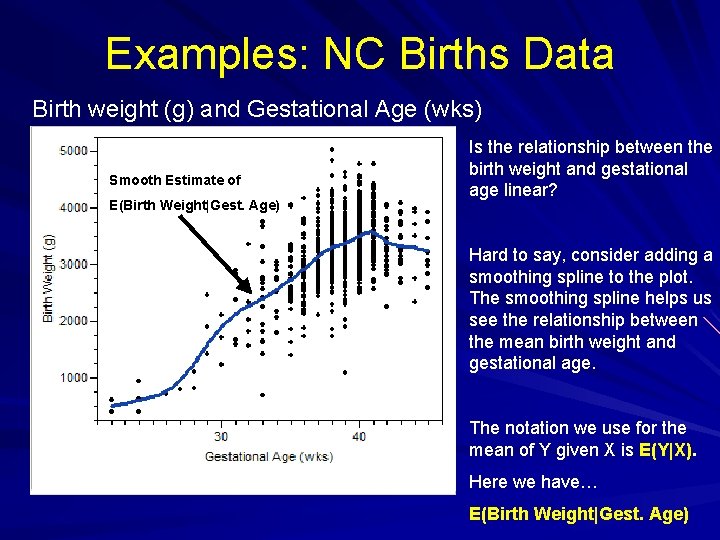
Examples: NC Births Data Birth weight (g) and Gestational Age (wks) Smooth Estimate of E(Birth Weight|Gest. Age) Is the relationship between the birth weight and gestational age linear? Hard to say, consider adding a smoothing spline to the plot. The smoothing spline helps us see the relationship between the mean birth weight and gestational age. The notation we use for the mean of Y given X is E(Y|X). Here we have… E(Birth Weight|Gest. Age)

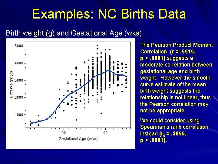
Examples: NC Births Data Birth weight (g) and Gestational Age (wks) The Pearson Product Moment Correlation (r =. 5515, p <. 0001) suggests a moderate correlation between gestational age and birth weight. However the smooth curve estimate of the mean birth weight suggests the relationship is not linear, thus the Pearson correlation may not be appropriate. We could consider using Spearman’s rank correlation instead (rs =. 3056, p <. 0001).

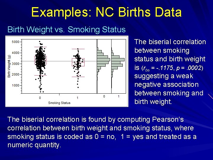
Examples: NC Births Data Birth Weight vs. Smoking Status The biserial correlation between smoking status and birth weight is (rbs = -. 1175, p =. 0002) suggesting a weak negative association between smoking and birth weight. The biserial correlation is found by computing Pearson’s correlation between birth weight and smoking status, where smoking status is coded as 0 = no, 1 = yes and treated as a numeric quantity.

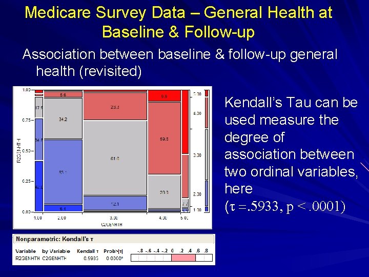
Medicare Survey Data – General Health at Baseline & Follow-up Association between baseline & follow-up general health (revisited) Kendall’s Tau can be used measure the degree of association between two ordinal variables, here (t . 5933, p <. 0001)

Simple Linear Regression • Regression refers to the estimation of the mean of a response (Y) given information about single predictor X in case of simple regression or multiple X’s in the case of multiple regression. • We denote this mean as E(Y|X) in the case simple regression and E(Y|X 1, X 2, …, Xp) in the case multiple regression with p potential predictors.

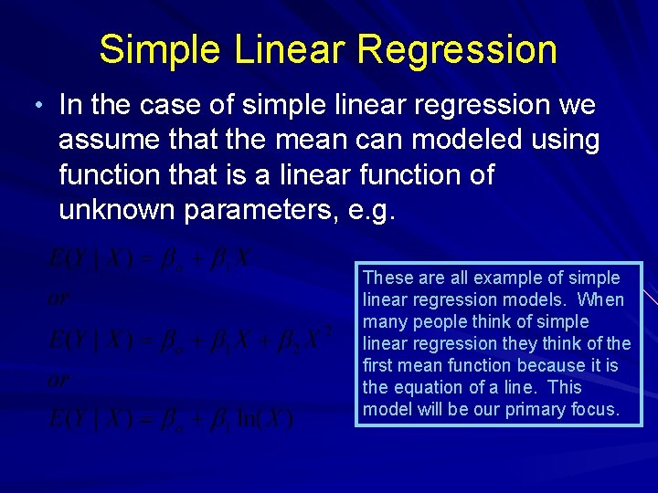
Simple Linear Regression • In the case of simple linear regression we assume that the mean can modeled using function that is a linear function of unknown parameters, e. g. These are all example of simple linear regression models. When many people think of simple linear regression they think of the first mean function because it is the equation of a line. This model will be our primary focus.

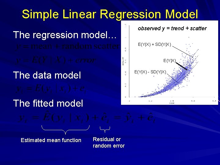
Simple Linear Regression Model The regression model… observed y = trend + scatter E(Y|X) + SD(Y|X) E(Y|X) - SD(Y|X) The data model The fitted model Estimated mean function Residual or random error

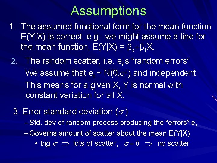
Assumptions 1. The assumed functional form for the mean function E(Y|X) is correct, e. g. we might assume a line for the mean function, E(Y|X) = bo+b 1 X. 2. The random scatter, i. e. ei’s “random errors” We assume that ei ~ N(0, s 2) and independent. This means for a given X, Y is normal with constant variation for all X. 3. Error standard deviation ( ) – Std. dev of random process producing the “errors” ei – Governs amount of scatter about the mean E(Y|X) • big lots of scatter, no scatter

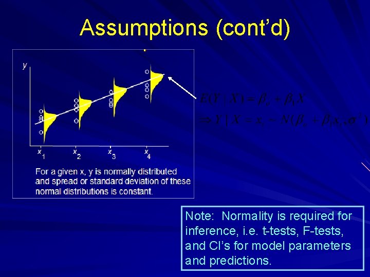
Assumptions (cont’d) Note: Normality is required for inference, i. e. t-tests, F-tests, and CI’s for model parameters and predictions.

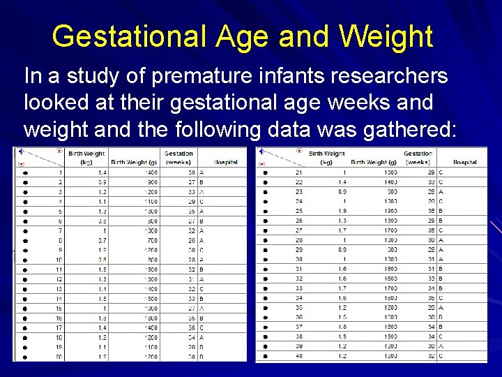
Gestational Age and Weight In a study of premature infants researchers looked at their gestational age weeks and weight and the following data was gathered:

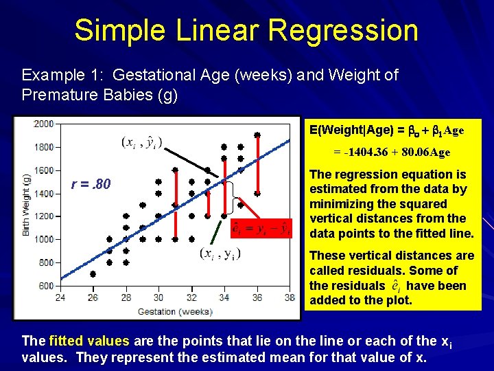
Simple Linear Regression Example 1: Gestational Age (weeks) and Weight of Premature Babies (g) E(Weight|Age) = bo + b 1 Age = -1404. 36 + 80. 06 Age r =. 80 The regression equation is estimated from the data by minimizing the squared vertical distances from the data points to the fitted line. These vertical distances are called residuals. Some of the residuals have been added to the plot. The fitted values are the points that lie on the line or each of the xi values. They represent the estimated mean for that value of x.

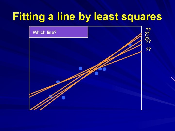
Fitting a line by least squares Which line? ? ? ? ? ?

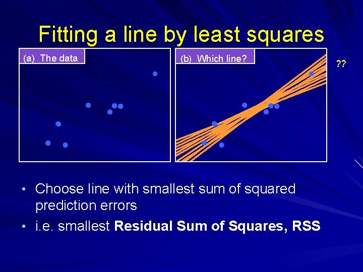
Fitting a line by least squares (a) The data (b) Which line? • Choose line with smallest sum of squared prediction errors • i. e. smallest Residual Sum of Squares, RSS ? ?

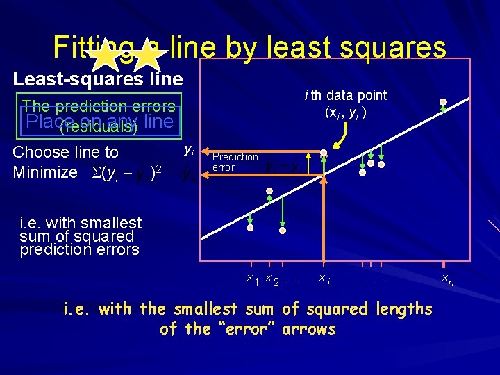
Fitting a line by least squares Least-squares line i th data point (xi , yi ) The prediction errors Place on any line (residuals) Choose line to Minimize S(yi - yi )2 Prediction error i. e. with smallest sum of squared prediction errors x 1 x 2. . xi . . . i. e. with the smallest sum of squared lengths of the “error” arrows xn

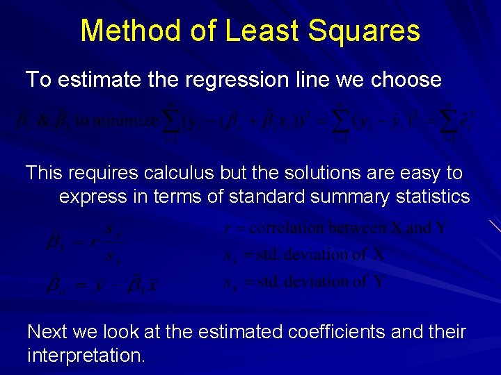
Method of Least Squares To estimate the regression line we choose This requires calculus but the solutions are easy to express in terms of standard summary statistics Next we look at the estimated coefficients and their interpretation.

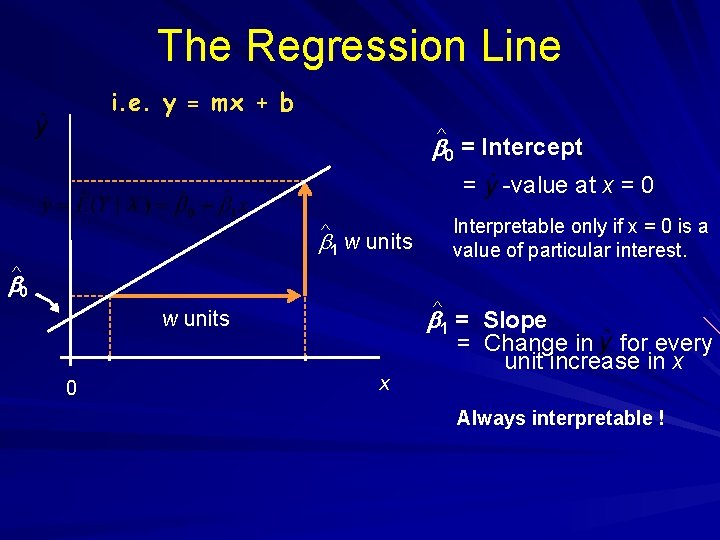
The Regression Line i. e. y = mx + b ^ b 0 = Intercept = -value at x = 0 Interpretable only if x = 0 is a value of particular interest. ^ b 1 w units ^ b 0 ^ b 1 = Slope w units 0 x = Change in for every unit increase in x Always interpretable !

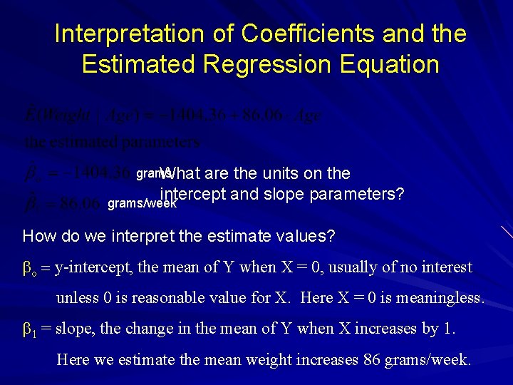
Interpretation of Coefficients and the Estimated Regression Equation grams What are the units on the intercept and slope parameters? grams/week How do we interpret the estimate values? bo y-intercept, the mean of Y when X = 0, usually of no interest unless 0 is reasonable value for X. Here X = 0 is meaningless. b 1 = slope, the change in the mean of Y when X increases by 1. Here we estimate the mean weight increases 86 grams/week.

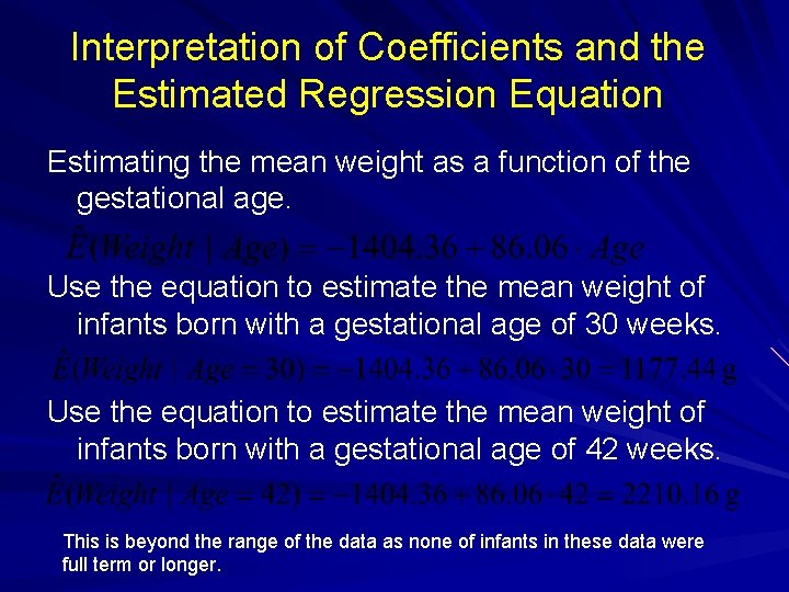
Interpretation of Coefficients and the Estimated Regression Equation Estimating the mean weight as a function of the gestational age. Use the equation to estimate the mean weight of infants born with a gestational age of 30 weeks. Use the equation to estimate the mean weight of infants born with a gestational age of 42 weeks. This is beyond the range of the data as none of infants in these data were full term or longer.

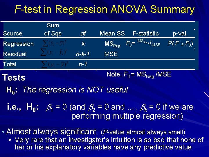
F-test in Regression ANOVA Summary Source Regression Residual Total Tests Sum of Sqs df k n-k-1 Mean SS F-statistic MSReg F 0= MSReg / MSE p-val. P( F F 0) MSE n-1 Note: F 0 = MSReg /MSE H 0: The regression is NOT useful i. e. , H 0: b 1 = 0 (and b 2 = 0 and …. bk = 0 if we are performing multiple regression) • Almost always significant (P-value almost always small) • Very rare that an investigator’s intuition is so bad that none of her or his explanatory variables have any predictive value

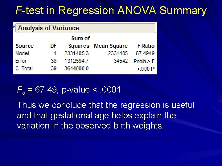
F-test in Regression ANOVA Summary Fo = 67. 49, p-value <. 0001 Thus we conclude that the regression is useful and that gestational age helps explain the variation in the observed birth weights.

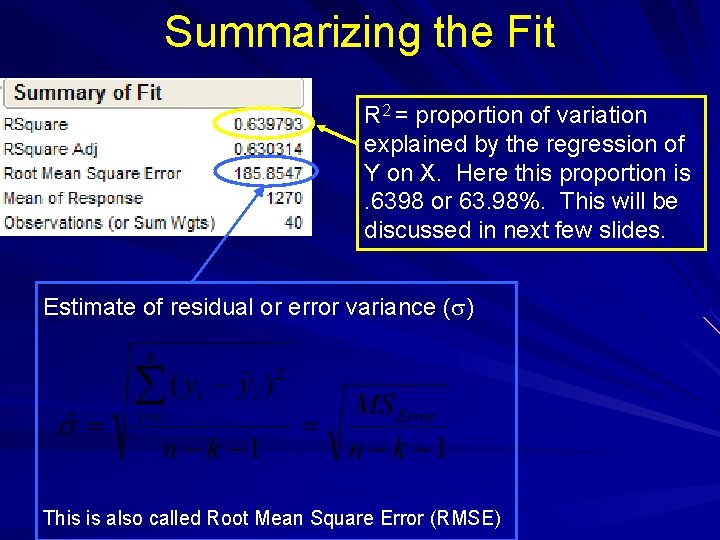
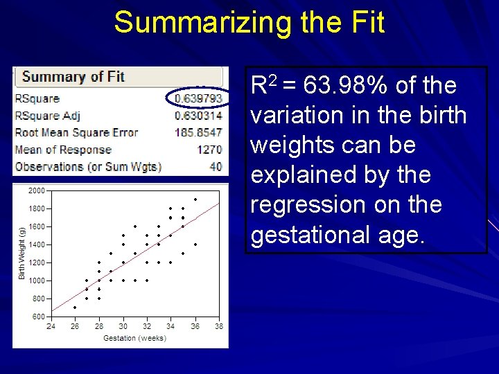
Summarizing the Fit R 2 = proportion of variation explained by the regression of Y on X. Here this proportion is. 6398 or 63. 98%. This will be discussed in next few slides. Estimate of residual or error variance (s) This is also called Root Mean Square Error (RMSE)

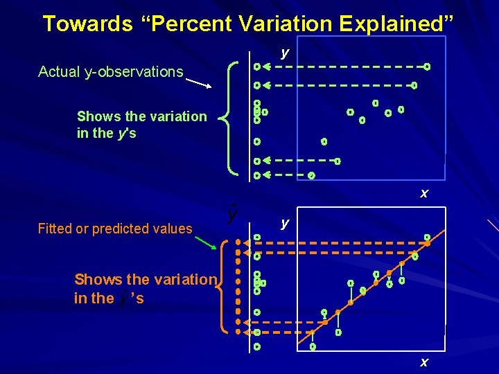
Towards “Percent Variation Explained” y Actual y-observations Shows the variation in the y's x Fitted or predicted values y Shows the variation in the ’s x

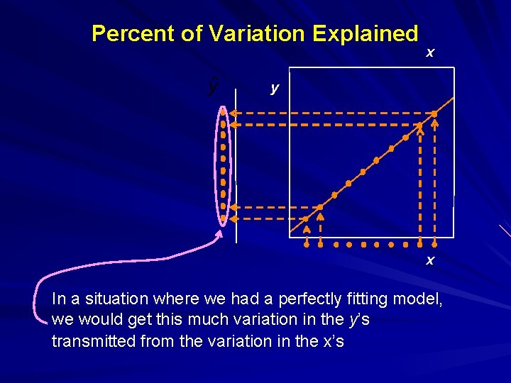
Percent of Variation Explained x y x In a situation where we had a perfectly fitting model, we would get this much variation in the y’s transmitted from the variation in the x’s

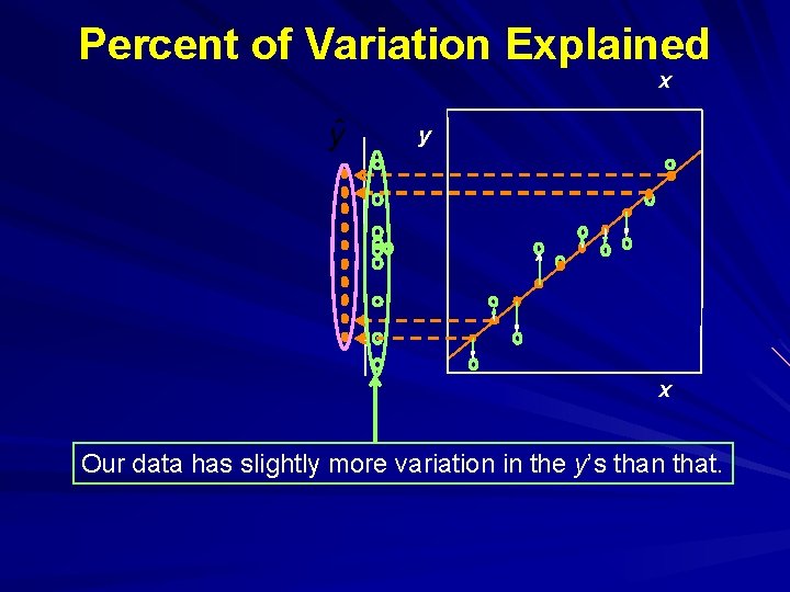
Percent of Variation Explained x y x Our data has slightly more variation in the y’s than that.

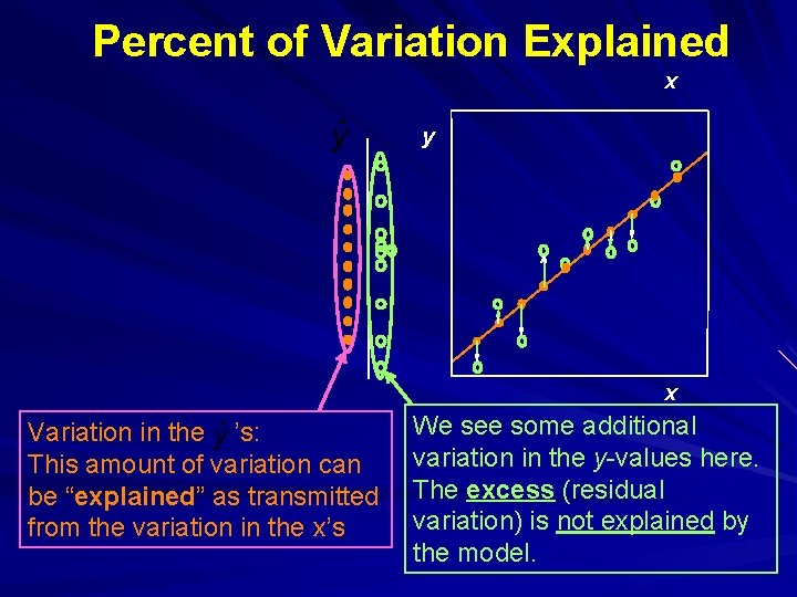
Percent of Variation Explained x y x Variation in the ’s: This amount of variation can be “explained” as transmitted from the variation in the x’s We see some additional variation in the y-values here. The excess (residual variation) is not explained by the model.

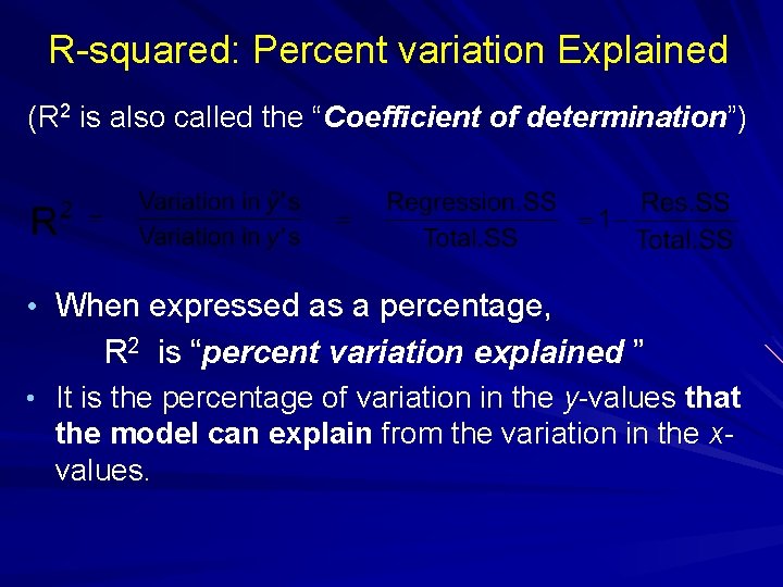
R-squared: Percent variation Explained (R 2 is also called the “Coefficient of determination”) • When expressed as a percentage, R 2 is “percent variation explained ” • It is the percentage of variation in the y-values that the model can explain from the variation in the xvalues.

Summarizing the Fit R 2 = 63. 98% of the variation in the birth weights can be explained by the regression on the gestational age.

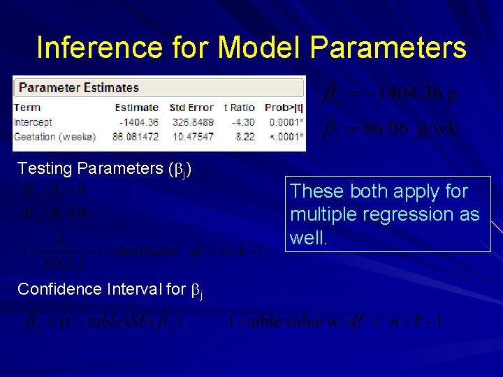
Inference for Model Parameters Testing Parameters (bj) Confidence Interval for bj These both apply for multiple regression as well.

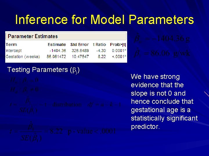
Inference for Model Parameters Testing Parameters (bj) We have strong evidence that the slope is not 0 and hence conclude that gestational age is a statistically significant predictor.

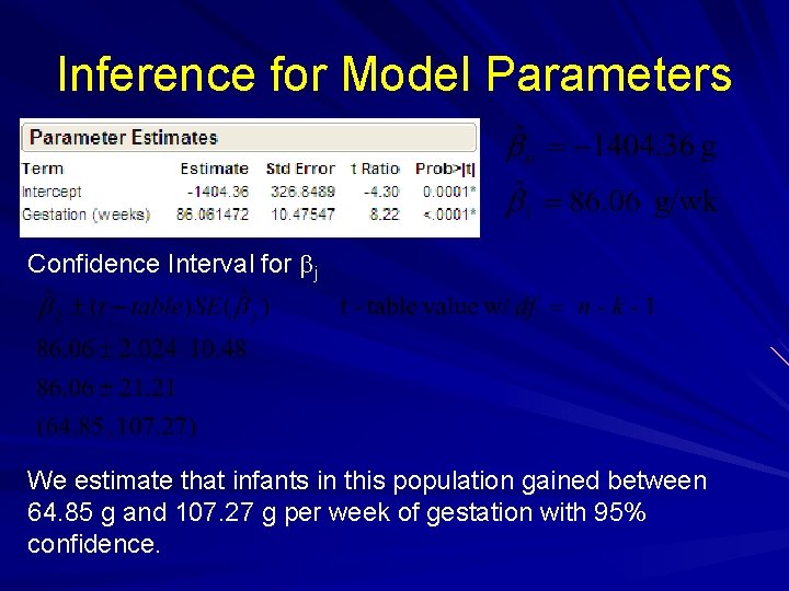
Inference for Model Parameters Confidence Interval for bj We estimate that infants in this population gained between 64. 85 g and 107. 27 g per week of gestation with 95% confidence.

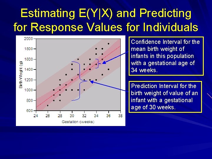
Estimating E(Y|X) and Predicting for Response Values for Individuals • We can construct CI’s for the mean of Y for a given value of X or for an individual with a given value of X. For the latter case we refer to the interval as a prediction interval (PI). • Both intervals we use the same point estimate from the regression equation as the center of the confidence interval.

Estimating E(Y|X) and Predicting for Response Values for Individuals Confidence Interval for the mean birth weight of infants in this population with a gestational age of 34 weeks. Prediction Interval for the birth weight of value of an infant with a gestational age of 30 weeks.

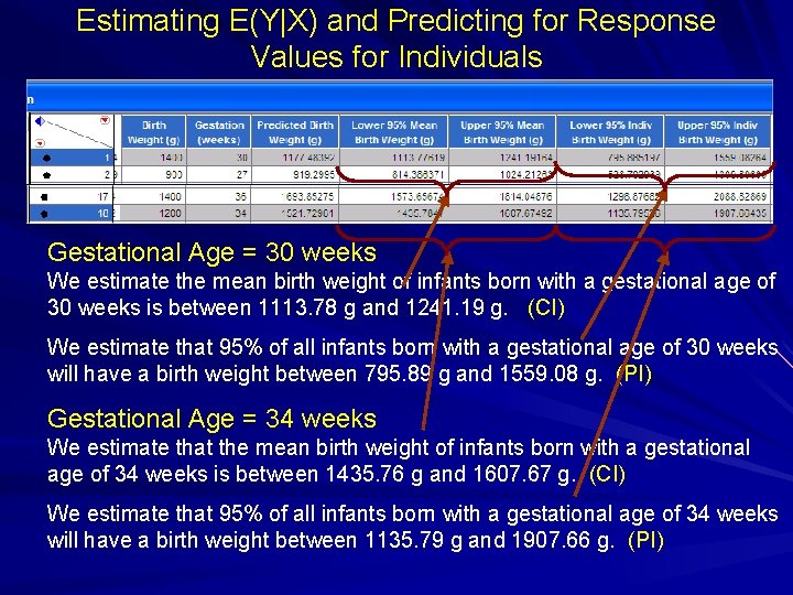
Estimating E(Y|X) and Predicting for Response Values for Individuals Gestational Age = 30 weeks We estimate the mean birth weight of infants born with a gestational age of 30 weeks is between 1113. 78 g and 1241. 19 g. (CI) We estimate that 95% of all infants born with a gestational age of 30 weeks will have a birth weight between 795. 89 g and 1559. 08 g. (PI) Gestational Age = 34 weeks We estimate that the mean birth weight of infants born with a gestational age of 34 weeks is between 1435. 76 g and 1607. 67 g. (CI) We estimate that 95% of all infants born with a gestational age of 34 weeks will have a birth weight between 1135. 79 g and 1907. 66 g. (PI)

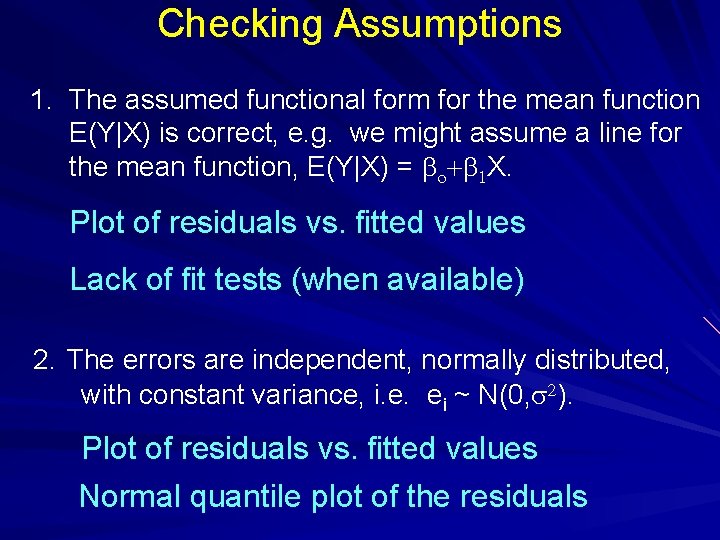
Checking Assumptions 1. The assumed functional form for the mean function E(Y|X) is correct, e. g. we might assume a line for the mean function, E(Y|X) = bo+b 1 X. Plot of residuals vs. fitted values Lack of fit tests (when available) 2. The errors are independent, normally distributed, with constant variance, i. e. ei ~ N(0, s 2). Plot of residuals vs. fitted values Normal quantile plot of the residuals

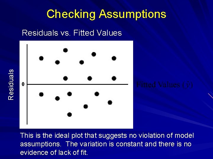
Checking Assumptions Residuals vs. Fitted Values 0 This is the ideal plot that suggests no violation of model assumptions. The variation is constant and there is no evidence of lack of fit.

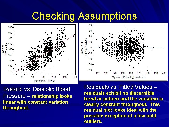
Checking Assumptions Systolic vs. Diastolic Blood Pressure – relationship looks linear with constant variation throughout. Residuals vs. Fitted Values – residuals exhibit no discernible trend or pattern and the variation is clearly constant throughout. This residual plot looks ideal with the possible exception of a few mild outliers.

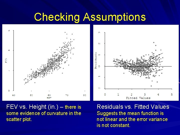
Checking Assumptions FEV vs. Height (in. ) – there is Residuals vs. Fitted Values some evidence of curvature in the scatter plot. Suggests the mean function is not linear and the error variance is not constant.

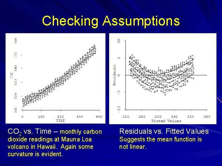
Checking Assumptions CO 2 vs. Time – monthly carbon dioxide readings at Mauna Loa volcano in Hawaii. Again some curvature is evident. Residuals vs. Fitted Values Suggests the mean function is not linear.

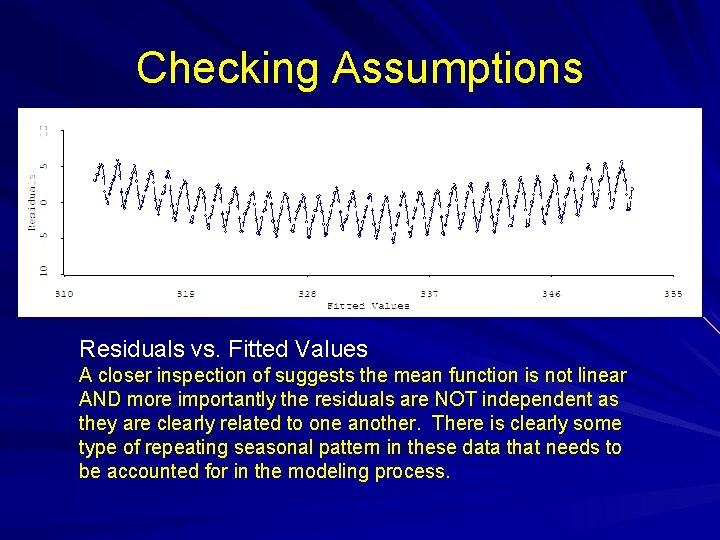
Checking Assumptions Residuals vs. Fitted Values A closer inspection of suggests the mean function is not linear AND more importantly the residuals are NOT independent as they are clearly related to one another. There is clearly some type of repeating seasonal pattern in these data that needs to be accounted for in the modeling process.

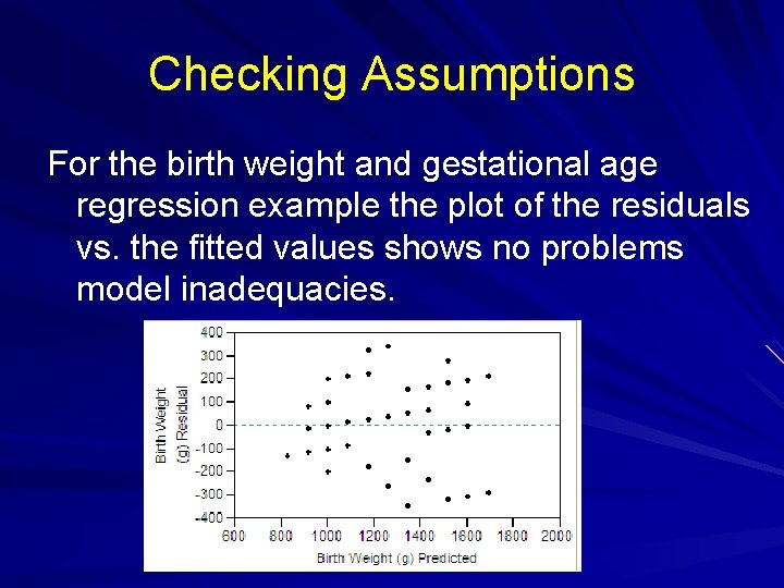
Checking Assumptions For the birth weight and gestational age regression example the plot of the residuals vs. the fitted values shows no problems model inadequacies.

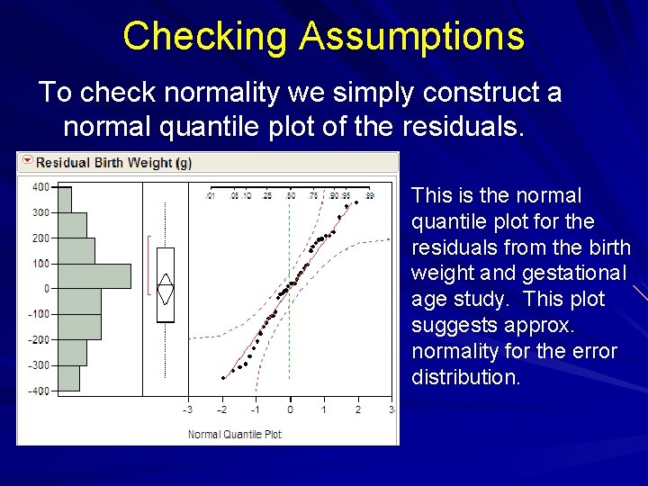
Checking Assumptions To check normality we simply construct a normal quantile plot of the residuals. This is the normal quantile plot for the residuals from the birth weight and gestational age study. This plot suggests approx. normality for the error distribution.

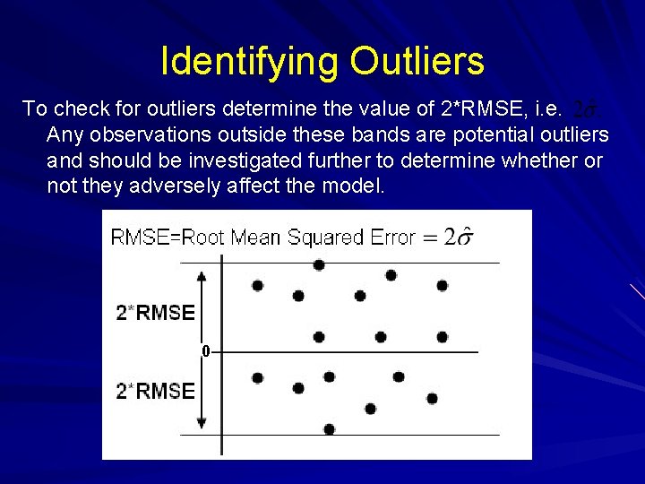
Identifying Outliers To check for outliers determine the value of 2*RMSE, i. e. Any observations outside these bands are potential outliers and should be investigated further to determine whether or not they adversely affect the model. 0

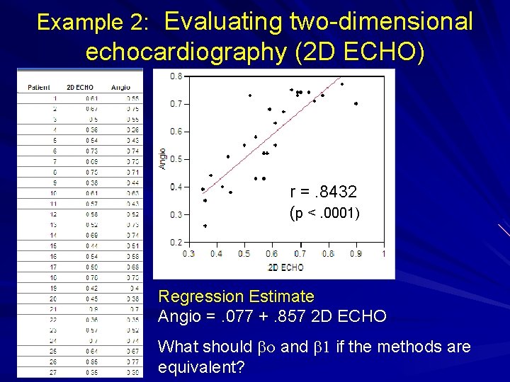
Example 2: Evaluating two-dimensional echocardiography (2 D ECHO) A study evaluated 2 D ECHO for the assessment of left ventricular diastolic filling. Data was collected on half-filling fraction (1/2 FF) for 27 patients as determined by both 2 D ECHO and angiography using diagnostic cardiac catheterization. Q: Do these data provide evidence that 1/2 FF obtained from angiography and 2 D ECHO are not equivalent?

Example 2: Evaluating two-dimensional echocardiography (2 D ECHO) r =. 8432 (p <. 0001) Regression Estimate Angio =. 077 +. 857 2 D ECHO What should bo and b 1 if the methods are equivalent?

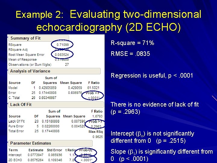
Example 2: Evaluating two-dimensional echocardiography (2 D ECHO) R-square = 71% RMSE =. 0835 Regression is useful, p <. 0001 There is no evidence of lack of fit (p =. 2963) Intercept (bo) is not significantly different from 0 (p =. 2515) Slope (b 1) is significantly different from 0 (p <. 0001)

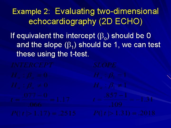
Example 2: Evaluating two-dimensional echocardiography (2 D ECHO) If equivalent the intercept (bo) should be 0 and the slope (b 1) should be 1, we can test these using the t-test.

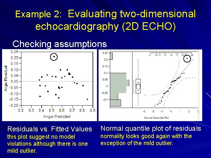
Example 2: Evaluating two-dimensional echocardiography (2 D ECHO) Checking assumptions Residuals vs. Fitted Values this plot suggest no model violations although there is one mild outlier. Normal quantile plot of residuals normality looks good again with the exception of the mild outlier.

Example 2: Evaluating two-dimensional echocardiography (2 D ECHO) Because we fail to reject the null hypothesis for both parameters we have no evidence against equality of the two methods for determining the half-filling fraction (1/2 FF). What other methods could be used to answer the question of interest? • Dependent samples t-test (paired t-test) • Wilcoxon signed rank test • Sign test (definitely the worst choice)

Summary • Type of correlation measure depends on - data types of X and Y - nature of the relationship (linear? ) • Simple Linear Regression - estimate the E(Y|X) - E(Y|X) need not a be line - be sure to check assumptions - variety of inferential methods • If assumptions are violated we need to change model or transform X and/or Y.