Constraint Program Solvers 600 325425 Declarative Methods J

Constraint Program Solvers 600. 325/425 Declarative Methods - J. Eisner 1

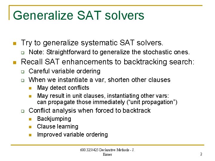
Generalize SAT solvers n Try to generalize systematic SAT solvers. q n Note: Straightforward to generalize the stochastic ones. Recall SAT enhancements to backtracking search: q q Careful variable ordering When we instantiate a var, shorten other clauses n n q May detect conflicts May result in unit clauses, instantiating other vars: can propagate those immediately (“unit propagation”) Conflict analysis when forced to backtrack n n n Backjumping Clause learning Improved variable ordering 600. 325/425 Declarative Methods - J. Eisner 2

Andrew Moore’s animations Graph coloring: Color every vertex so that adjacent vertices have different colors. (NP-complete, many applications such as register allocation) http: //www-2. cs. cmu. edu/~awm/animations/constraint/ 600. 325/425 Declarative Methods - J. Eisner 3

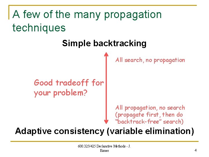
A few of the many propagation techniques Simple backtracking All search, no propagation Good tradeoff for your problem? All propagation, no search (propagate first, then do “backtrack-free” search) Adaptive consistency (variable elimination) 600. 325/425 Declarative Methods - J. Eisner 4

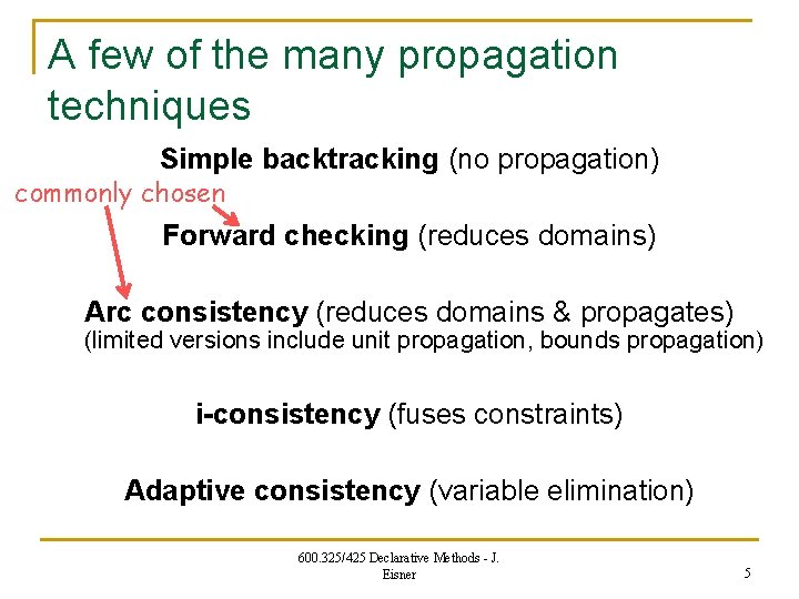
A few of the many propagation techniques Simple backtracking (no propagation) commonly chosen Forward checking (reduces domains) Arc consistency (reduces domains & propagates) (limited versions include unit propagation, bounds propagation) i-consistency (fuses constraints) Adaptive consistency (variable elimination) 600. 325/425 Declarative Methods - J. Eisner 5

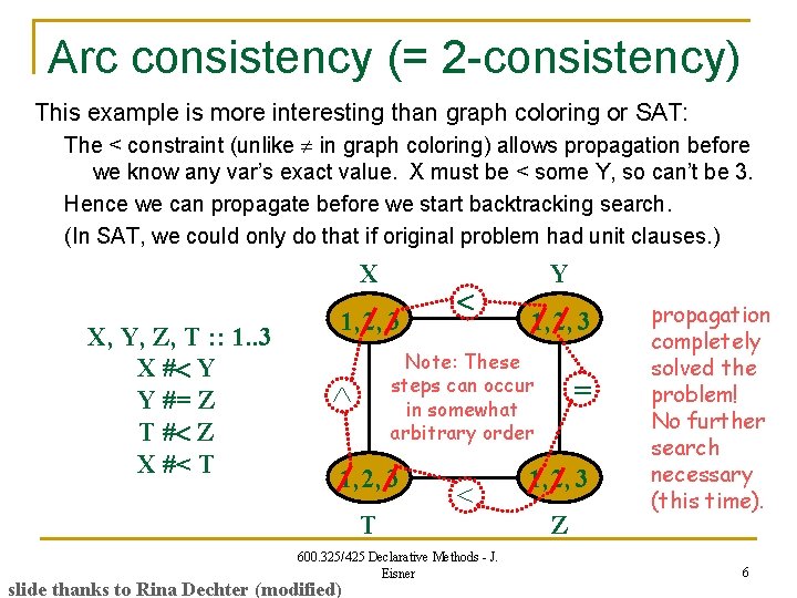
Arc consistency (= 2 -consistency) This example is more interesting than graph coloring or SAT: The < constraint (unlike in graph coloring) allows propagation before we know any var’s exact value. X must be < some Y, so can’t be 3. Hence we can propagate before we start backtracking search. (In SAT, we could only do that if original problem had unit clauses. ) X X, Y, Z, T : : 1. . 3 X # Y Y #= Z T # Z X #< T 1, 2, 3 Note: These steps can occur in somewhat arbitrary order 1, 2, 3 T 600. 325/425 Declarative Methods - J. Eisner slide thanks to Rina Dechter (modified) Y = 1, 2, 3 Z propagation completely solved the problem! No further search necessary (this time). 6

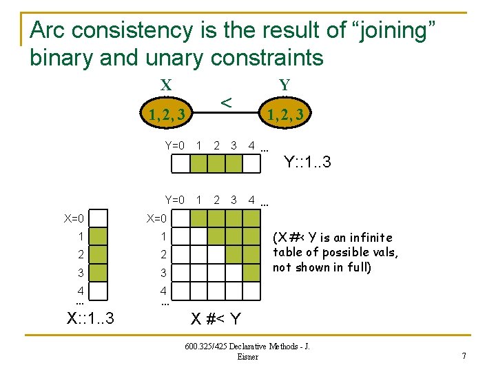
Arc consistency is the result of “joining” binary and unary constraints X 1, 2, 3 Y=0 1 X=0 1 1 2 2 3 3 4 … X: : 1. . 3 2 2 3 3 Y 1, 2, 3 4 … Y: : 1. . 3 4 … (X #< Y is an infinite table of possible vals, not shown in full) 4 … X #< Y 600. 325/425 Declarative Methods - J. Eisner 7

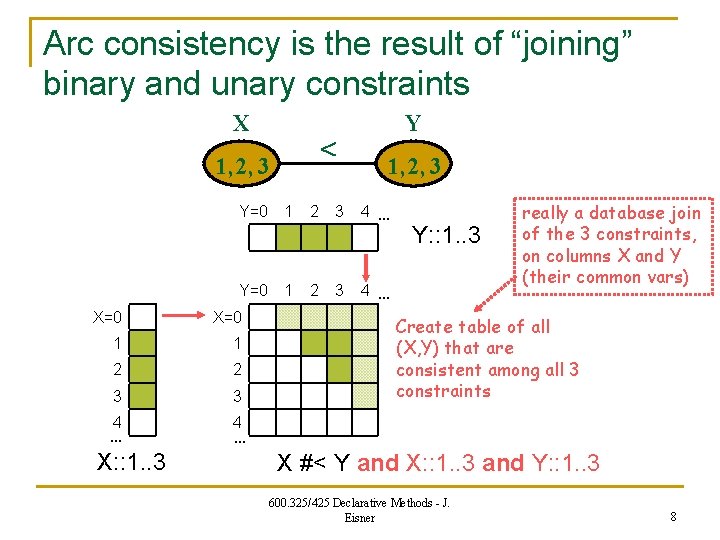
Arc consistency is the result of “joining” binary and unary constraints X 1, 2, 3 Y=0 1 X=0 1 1 2 2 3 3 4 … X: : 1. . 3 2 2 3 3 Y 1, 2, 3 4 … Y: : 1. . 3 4 … really a database join of the 3 constraints, on columns X and Y (their common vars) Create table of all (X, Y) that are consistent among all 3 constraints 4 … X #< Y and X: : 1. . 3 and Y: : 1. . 3 600. 325/425 Declarative Methods - J. Eisner 8

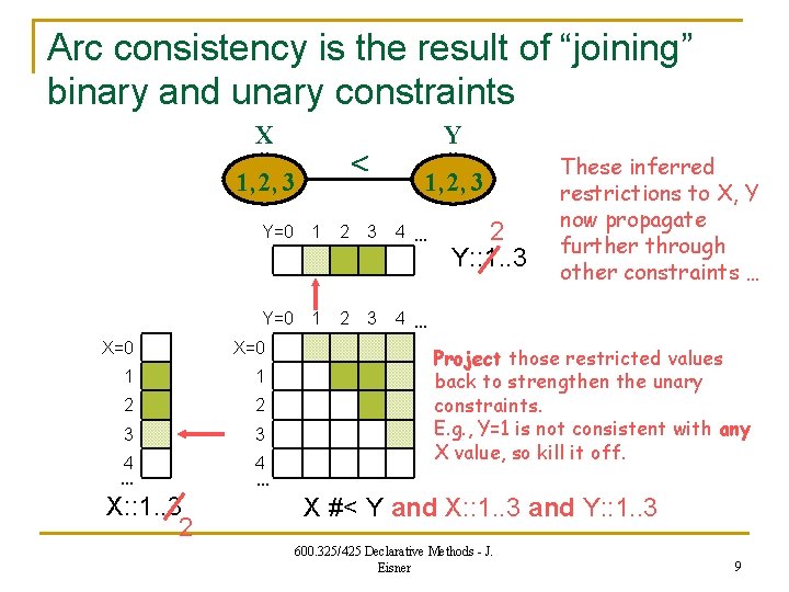
Arc consistency is the result of “joining” binary and unary constraints X 1, 2, 3 2 3 4 … Y=0 1 2 3 4 … X=0 1 1 2 2 3 3 4 X: : 1. . 3 2 1, 2, 3 Y=0 1 X=0 … Y 4 … 2 Y: : 1. . 3 These inferred restrictions to X, Y now propagate further through other constraints … Project those restricted values back to strengthen the unary constraints. E. g. , Y=1 is not consistent with any X value, so kill it off. X #< Y and X: : 1. . 3 and Y: : 1. . 3 600. 325/425 Declarative Methods - J. Eisner 9

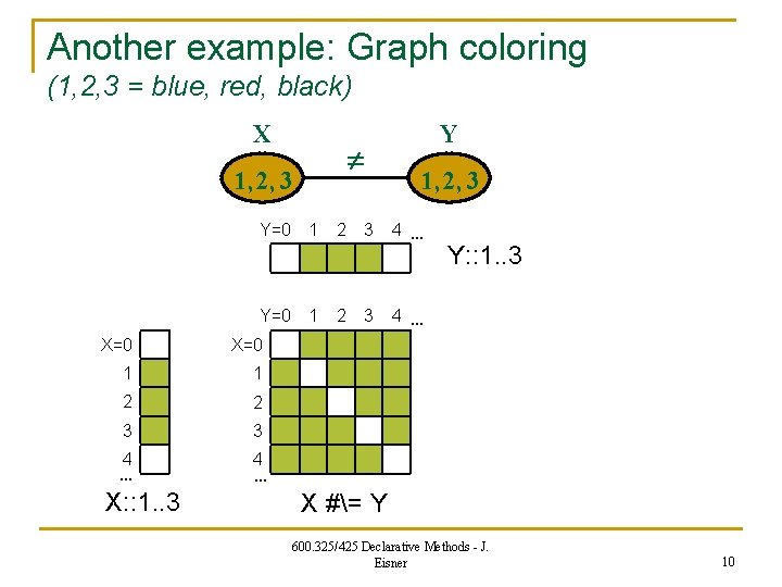
Another example: Graph coloring (1, 2, 3 = blue, red, black) X 1, 2, 3 Y=0 1 X=0 1 1 2 2 3 3 4 … X: : 1. . 3 2 2 3 3 Y 1, 2, 3 4 … Y: : 1. . 3 4 … X #= Y 600. 325/425 Declarative Methods - J. Eisner 10

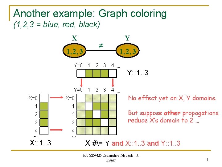
Another example: Graph coloring (1, 2, 3 = blue, red, black) X 1, 2, 3 Y=0 1 X=0 1 1 2 2 3 3 4 … X: : 1. . 3 2 2 3 3 Y 1, 2, 3 4 … Y: : 1. . 3 No effect yet on X, Y domains. But suppose other propagations reduce X’s domain to 2 … 4 … X #= Y and X: : 1. . 3 and Y: : 1. . 3 600. 325/425 Declarative Methods - J. Eisner 11

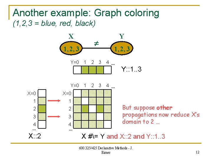
Another example: Graph coloring (1, 2, 3 = blue, red, black) X 1, 2, 3 Y=0 1 X=0 1 1 2 2 3 3 4 … X: : 2 4 … 2 2 3 3 Y 1, 2, 3 4 … Y: : 1. . 3 4 … But suppose other propagations now reduce X’s domain to 2 … X #= Y and X: : 2 and Y: : 1. . 3 600. 325/425 Declarative Methods - J. Eisner 12

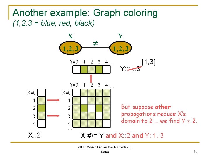
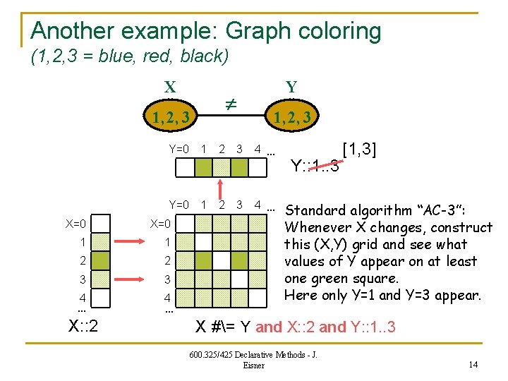
Another example: Graph coloring (1, 2, 3 = blue, red, black) X 1, 2, 3 Y=0 1 X=0 1 1 2 2 3 3 4 … X: : 2 4 … 2 2 3 3 Y 1, 2, 3 4 … Y: : 1. . 3 [1, 3] 4 … But suppose other propagations reduce X’s domain to 2 … we find Y 2. X #= Y and X: : 2 and Y: : 1. . 3 600. 325/425 Declarative Methods - J. Eisner 13

Another example: Graph coloring (1, 2, 3 = blue, red, black) X 1, 2, 3 Y=0 1 X=0 1 1 2 2 3 3 4 … X: : 2 4 … 2 2 3 3 Y 1, 2, 3 4 … Y: : 1. . 3 [1, 3] Standard algorithm “AC-3”: Whenever X changes, construct this (X, Y) grid and see what values of Y appear on at least one green square. Here only Y=1 and Y=3 appear. X #= Y and X: : 2 and Y: : 1. . 3 600. 325/425 Declarative Methods - J. Eisner 14

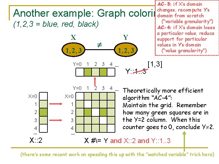
AC-3: if X’s domain changes, recompute Y’s domain from scratch (“variable granularity”) AC-4: if X’s domain loses a particular value, reduce support for particular values in Y’s domain (“value granularity”) Another example: Graph coloring (1, 2, 3 = blue, red, black) X 1, 2, 3 Y=0 1 X=0 1 1 2 2 3 3 4 … X: : 2 4 … 2 2 3 3 Y 1, 2, 3 4 … Y: : 1. . 3 [1, 3] Theoretically more efficient algorithm “AC-4”: Maintain the grid. Remember how many green squares are in the Y=2 column. When this counter goes to 0, conclude Y 2. X #= Y and X: : 2 and Y: : 1. . 3 600. 325/425 Declarative Methods - J. (there’s some recent work on speeding this up with the “watched variable” trick 15 here) Eisner

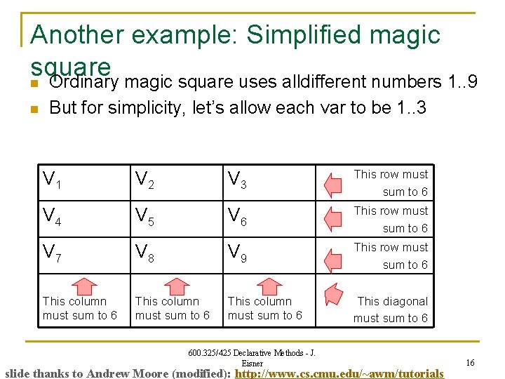
Another example: Simplified magic square n Ordinary magic square uses alldifferent numbers 1. . 9 n But for simplicity, let’s allow each var to be 1. . 3 V 1 V 2 V 3 This row must sum to 6 V 4 V 5 V 6 This row must sum to 6 V 7 V 8 V 9 This row must sum to 6 This column must sum to 6 This diagonal must sum to 6 600. 325/425 Declarative Methods - J. Eisner slide thanks to Andrew Moore (modified): http: //www. cs. cmu. edu/~awm/tutorials 16

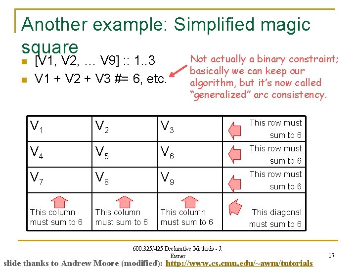
Another example: Simplified magic square Not actually a binary constraint; n n [V 1, V 2, … V 9] : : 1. . 3 V 1 + V 2 + V 3 #= 6, etc. basically we can keep our algorithm, but it’s now called “generalized” arc consistency. V 1 V 2 V 3 This row must sum to 6 V 4 V 5 V 6 This row must sum to 6 V 7 V 8 V 9 This row must sum to 6 This column must sum to 6 This diagonal must sum to 6 600. 325/425 Declarative Methods - J. Eisner slide thanks to Andrew Moore (modified): http: //www. cs. cmu. edu/~awm/tutorials 17

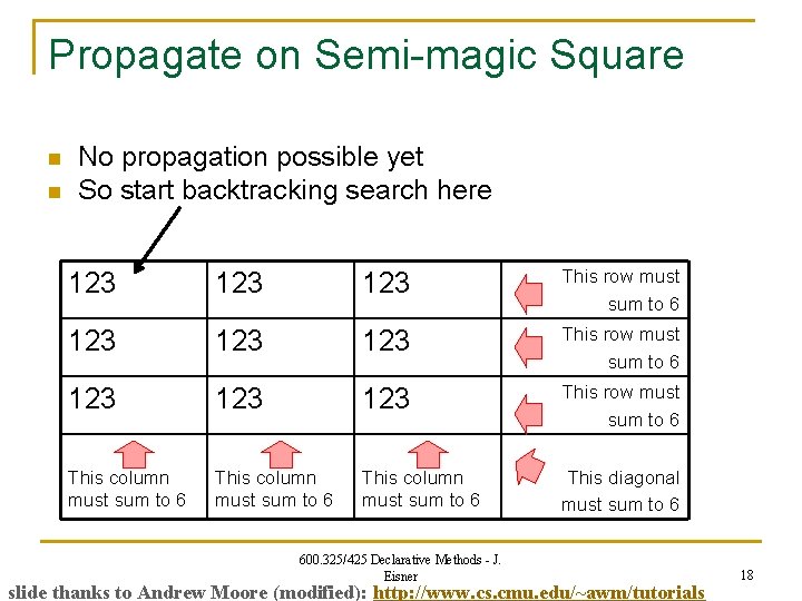
Propagate on Semi-magic Square n n No propagation possible yet So start backtracking search here 123 123 123 This row must sum to 6 This column must sum to 6 This diagonal must sum to 6 600. 325/425 Declarative Methods - J. Eisner slide thanks to Andrew Moore (modified): http: //www. cs. cmu. edu/~awm/tutorials 18

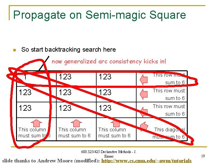
Propagate on Semi-magic Square n So start backtracking search here now generalized arc consistency kicks in! 1 123 123 This row must sum to 6 This column must sum to 6 This diagonal must sum to 6 600. 325/425 Declarative Methods - J. Eisner slide thanks to Andrew Moore (modified): http: //www. cs. cmu. edu/~awm/tutorials 19

Propagate on Semi-magic Square n So start backtracking search here any further propagation from these changes? 1 23 23 This row must sum to 6 23 23 123 This row must sum to 6 23 123 23 This row must sum to 6 This column must sum to 6 This diagonal must sum to 6 600. 325/425 Declarative Methods - J. Eisner slide thanks to Andrew Moore (modified): http: //www. cs. cmu. edu/~awm/tutorials 20

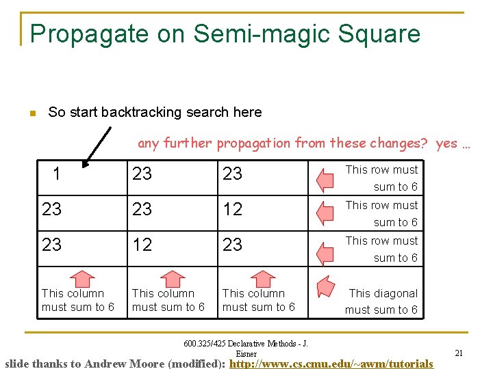
Propagate on Semi-magic Square n So start backtracking search here any further propagation from these changes? yes … 1 23 23 This row must sum to 6 23 23 12 This row must sum to 6 23 12 23 This row must sum to 6 This column must sum to 6 This diagonal must sum to 6 600. 325/425 Declarative Methods - J. Eisner slide thanks to Andrew Moore (modified): http: //www. cs. cmu. edu/~awm/tutorials 21

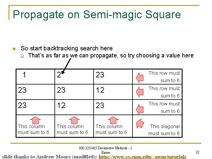
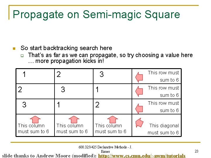
Propagate on Semi-magic Square n So start backtracking search here q That’s as far as we can propagate, so try choosing a value here 1 2 23 This row must sum to 6 23 23 12 This row must sum to 6 23 12 23 This row must sum to 6 This column must sum to 6 This diagonal must sum to 6 600. 325/425 Declarative Methods - J. Eisner slide thanks to Andrew Moore (modified): http: //www. cs. cmu. edu/~awm/tutorials 22

Propagate on Semi-magic Square n So start backtracking search here q That’s as far as we can propagate, so try choosing a value here … more propagation kicks in! 1 2 3 This column must sum to 6 2 3 This row must sum to 6 1 2 This row must sum to 6 This column must sum to 6 This diagonal must sum to 6 3 600. 325/425 Declarative Methods - J. Eisner slide thanks to Andrew Moore (modified): http: //www. cs. cmu. edu/~awm/tutorials 23

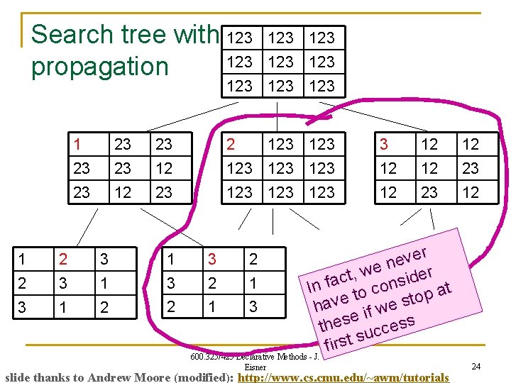
Search tree with 123 propagation 123 123 1 23 23 23 12 23 1 2 3 1 3 1 2 123 3 12 12 123 123 12 12 23 123 12 ver e n we ider , t c 3 2 1 In fa to cons p at o t e s v a e 2 1 3 h if w s e s the ucces if rst s 600. 325/425 Declarative Methods - J. 1 3 2 Eisner slide thanks to Andrew Moore (modified): http: //www. cs. cmu. edu/~awm/tutorials 24

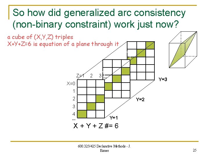
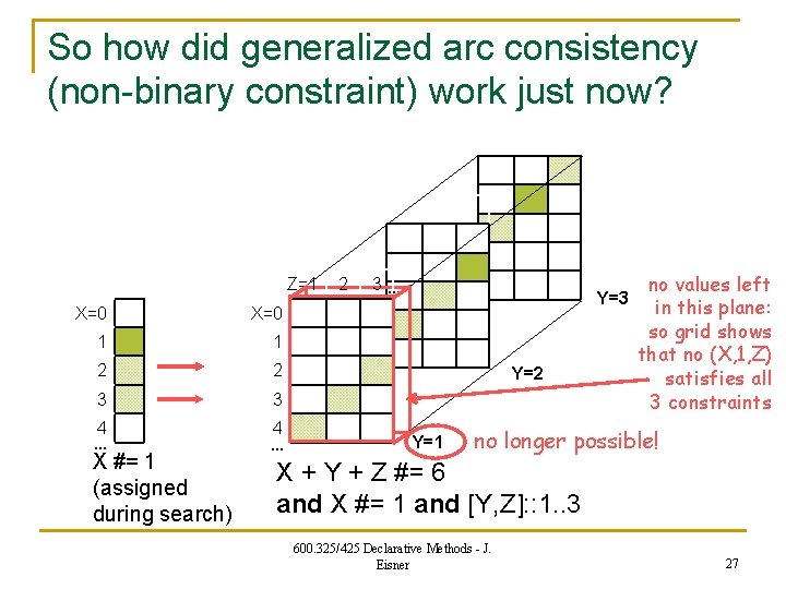
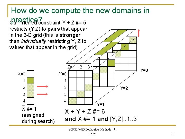
So how did generalized arc consistency (non-binary constraint) work just now? a cube of (X, Y, Z) triples X+Y+Z=6 is equation of a plane through it Z=1 2 3… Y=3 X=0 1 2 Y=2 3 4 … Y=1 X + Y + Z #= 6 600. 325/425 Declarative Methods - J. Eisner 25

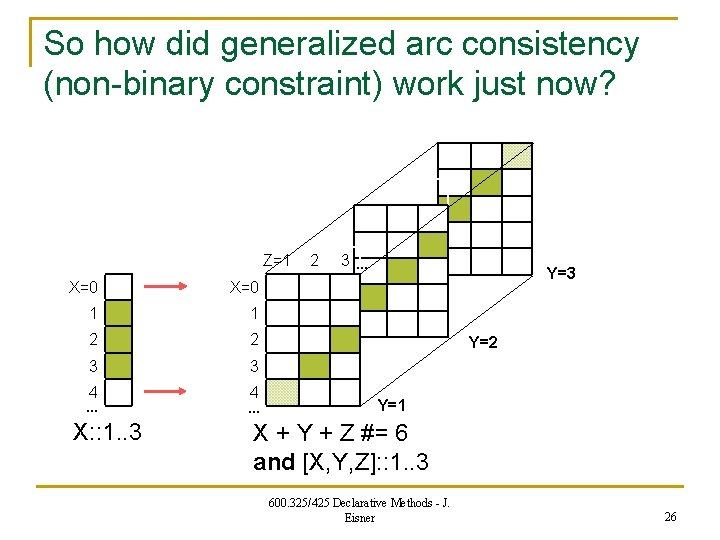
So how did generalized arc consistency (non-binary constraint) work just now? Z=1 X=0 1 1 2 2 3 3 4 … X: : 1. . 3 4 … 2 3… Y=3 Y=2 Y=1 X + Y + Z #= 6 and [X, Y, Z]: : 1. . 3 600. 325/425 Declarative Methods - J. Eisner 26

So how did generalized arc consistency (non-binary constraint) work just now? Z=1 X=0 1 1 2 2 3 3 4 … X #= 1 (assigned during search) 4 … 2 3… Y=3 Y=2 Y=1 no values left in this plane: so grid shows that no (X, 1, Z) satisfies all 3 constraints no longer possible! X + Y + Z #= 6 and X #= 1 and [Y, Z]: : 1. . 3 600. 325/425 Declarative Methods - J. Eisner 27

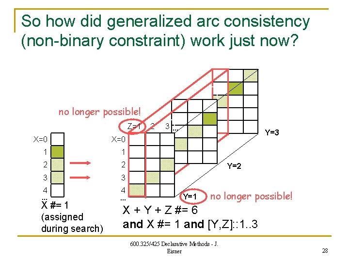
So how did generalized arc consistency (non-binary constraint) work just now? no longer possible! Z=1 X=0 1 1 2 2 3 3 4 … X #= 1 (assigned during search) 4 … 2 3… Y=3 Y=2 Y=1 no longer possible! X + Y + Z #= 6 and X #= 1 and [Y, Z]: : 1. . 3 600. 325/425 Declarative Methods - J. Eisner 28

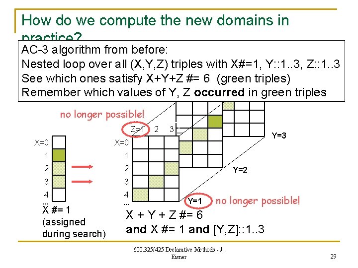
How do we compute the new domains in practice? AC-3 algorithm from before: Nested loop over all (X, Y, Z) triples with X#=1, Y: : 1. . 3, Z: : 1. . 3 See which ones satisfy X+Y+Z #= 6 (green triples) Remember which values of Y, Z occurred in green triples no longer possible! Z=1 X=0 1 1 2 2 3 3 4 … X #= 1 (assigned during search) 4 … 2 3… Y=3 Y=2 Y=1 no longer possible! X + Y + Z #= 6 and X #= 1 and [Y, Z]: : 1. . 3 600. 325/425 Declarative Methods - J. Eisner 29

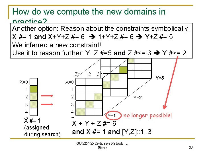
How do we compute the new domains in practice? Another option: Reason about the constraints symbolically! X #= 1 and X+Y+Z #= 6 1+Y+Z #= 6 Y+Z #= 5 We inferred a new constraint! Use it to reason further: Y+Z #=5 and Z #<= 3 Y #>= 2 Z=1 X=0 1 1 2 2 3 3 4 … X #= 1 (assigned during search) 4 … 2 3… Y=3 Y=2 Y=1 no longer possible! X + Y + Z #= 6 and X #= 1 and [Y, Z]: : 1. . 3 600. 325/425 Declarative Methods - J. Eisner 30

How do we compute the new domains in practice? Our inferred constraint Y + Z #= 5 restricts (Y, Z) to pairs that appear in the 3 -D grid (this is stronger than individually restricting Y, Z to values that appear in the grid) Z=1 X=0 1 1 2 2 3 3 4 … X #= 1 (assigned during search) 4 … 2 3… Y=3 Y=2 Y=1 X + Y + Z #= 6 and X #= 1 and [Y, Z]: : 1. . 3 600. 325/425 Declarative Methods - J. Eisner 31

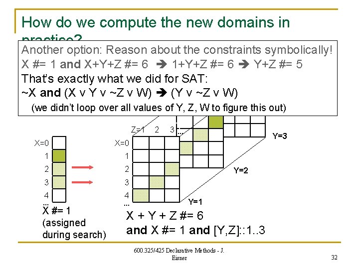
How do we compute the new domains in practice? Another option: Reason about the constraints symbolically! X #= 1 and X+Y+Z #= 6 1+Y+Z #= 6 Y+Z #= 5 That’s exactly what we did for SAT: ~X and (X v Y v ~Z v W) (Y v ~Z v W) (we didn’t loop over all values of Y, Z, W to figure this out) Z=1 X=0 1 1 2 2 3 3 4 … X #= 1 (assigned during search) 4 … 2 3… Y=3 Y=2 Y=1 X + Y + Z #= 6 and X #= 1 and [Y, Z]: : 1. . 3 600. 325/425 Declarative Methods - J. Eisner 32

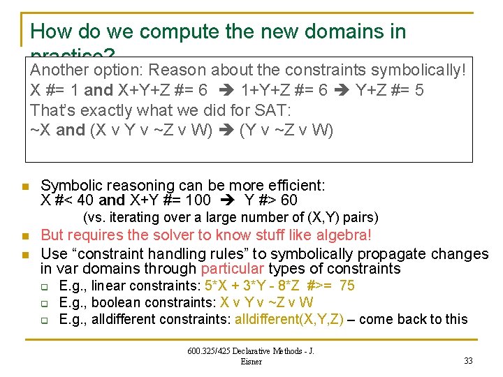
How do we compute the new domains in practice? Another option: Reason about the constraints symbolically! X #= 1 and X+Y+Z #= 6 1+Y+Z #= 6 Y+Z #= 5 That’s exactly what we did for SAT: ~X and (X v Y v ~Z v W) (Y v ~Z v W) n Symbolic reasoning can be more efficient: X #< 40 and X+Y #= 100 Y #> 60 (vs. iterating over a large number of (X, Y) pairs) n n But requires the solver to know stuff like algebra! Use “constraint handling rules” to symbolically propagate changes in var domains through particular types of constraints q q q E. g. , linear constraints: 5*X + 3*Y - 8*Z #>= 75 E. g. , boolean constraints: X v Y v ~Z v W E. g. , alldifferent constraints: alldifferent(X, Y, Z) – come back to this 600. 325/425 Declarative Methods - J. Eisner 33

Strong and weak propagators Designing good propagators (constraint handling rules) n q q Weak propagators run fast, but may not eliminate all impossible values from the variable domains. n q So backtracking search must consider & eliminate more values. Strong propagators work harder – not always worth it. n n a lot of the “art” of constraint solving the subject of the rest of the lecture Use “constraint handling rules” to symbolically propagate changes in var domains through particular types of constraints q q q E. g. , linear constraints: 5*X + 3*Y - 8*Z #>= 75 E. g. , boolean constraints: X v Y v ~Z v W E. g. , alldifferent constraints: alldifferent(X, Y, Z) – come back to this 600. 325/425 Declarative Methods - J. Eisner 34

Example of weak propagators: Bounds propagation for linear constraints n [A, B, C, D] : : 1. . 100 n n n A #= B (inequality) B + C #= 100 7*B + 3*D #> 50 B y Multiply: -7 B -7 y Add to: 7 B + 3 D > 50 Result: 3 D > 50 -7 y Therefore: D > (50 -7 y)/3 Might want to use a simple, weak propagator for these linear constraints: Revise C, D only if something changes B’s total range min(B). . max(B). If we learn that B x, for some const x, conclude C 100 -x If we learn that B y, conclude C 100 -y and D > (50+7 y)/3 So new lower/upper bounds on B give new bounds on C, D. That is, shrinking B’s range shrinks 600. 325/425 Declarative Methods - J. other variables’ ranges. Eisner 35

Example of weak propagators: Bounds propagation for linear constraints n [A, B, C, D] : : 1. . 100 A #= B (inequality) B + C #= 100 7*B + 3*D #> 50 Might want to use a simple, weak propagator for these linear constraints: n Revise C, D only if something changes B’s n total range min(B). . max(B). Why is this only a weak propagator? It does nothing if B gets a hole in the middle of its range. Suppose we discover or guess that A=75 Full arc consistency would propagate as follows: our bounds domain(A) changed – revise B : : 1. . 100 [1. . 74, 76. . 100] propagator domain(B) changed – revise C : : 1. . 100 [1. . 24, 26. . 100] doesn’t try domain(B) changed – revise D : : 1. . 100 to get these (wasted time figuring out there was no change) revisions. n 600. 325/425 Declarative Methods - J. Eisner 36

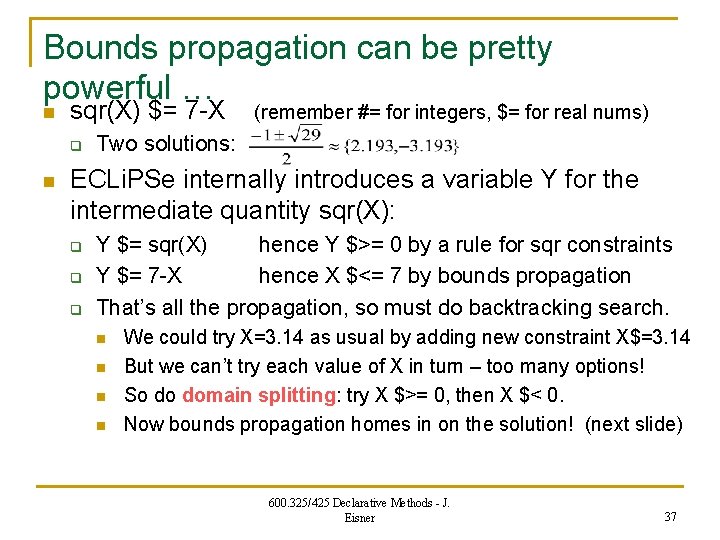
Bounds propagation can be pretty powerful … n sqr(X) $= 7 -X q n (remember #= for integers, $= for real nums) Two solutions: ECLi. PSe internally introduces a variable Y for the intermediate quantity sqr(X): q q q Y $= sqr(X) hence Y $>= 0 by a rule for sqr constraints Y $= 7 -X hence X $<= 7 by bounds propagation That’s all the propagation, so must do backtracking search. n n We could try X=3. 14 as usual by adding new constraint X$=3. 14 But we can’t try each value of X in turn – too many options! So do domain splitting: try X $>= 0, then X $< 0. Now bounds propagation homes in on the solution! (next slide) 600. 325/425 Declarative Methods - J. Eisner 37

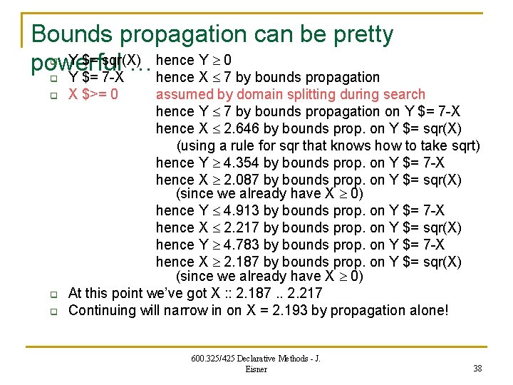
Bounds propagation can be pretty Y $= sqr(X) hence Y 0 powerful … Y $= 7 -X hence X 7 by bounds propagation q q q X $>= 0 assumed by domain splitting during search hence Y 7 by bounds propagation on Y $= 7 -X hence X 2. 646 by bounds prop. on Y $= sqr(X) (using a rule for sqr that knows how to take sqrt) hence Y 4. 354 by bounds prop. on Y $= 7 -X hence X 2. 087 by bounds prop. on Y $= sqr(X) (since we already have X 0) hence Y 4. 913 by bounds prop. on Y $= 7 -X hence X 2. 217 by bounds prop. on Y $= sqr(X) hence Y 4. 783 by bounds prop. on Y $= 7 -X hence X 2. 187 by bounds prop. on Y $= sqr(X) (since we already have X 0) At this point we’ve got X : : 2. 187. . 2. 217 Continuing will narrow in on X = 2. 193 by propagation alone! 600. 325/425 Declarative Methods - J. Eisner 38

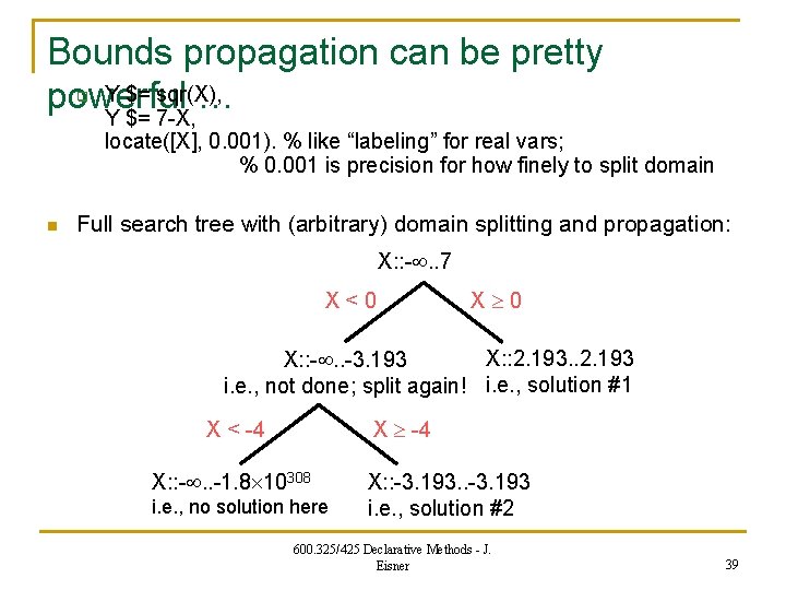
Bounds propagation can be pretty Y $= sqr(X), powerful … Y $= 7 -X, q locate([X], 0. 001). % like “labeling” for real vars; % 0. 001 is precision for how finely to split domain n Full search tree with (arbitrary) domain splitting and propagation: X: : -. . 7 X<0 X 0 X: : 2. 193. . 2. 193 X: : -. . -3. 193 i. e. , not done; split again! i. e. , solution #1 X -4 X < -4 X: : -. . -1. 8 10308 i. e. , no solution here X: : -3. 193. . -3. 193 i. e. , solution #2 600. 325/425 Declarative Methods - J. Eisner 39

Moving on … n We started with generalized arc consistency as our basic method. n Bounds consistency is weaker, but often effective (and more efficient) for arithmetic constraints. What is stronger than arc consistency? n 600. 325/425 Declarative Methods - J. Eisner 40

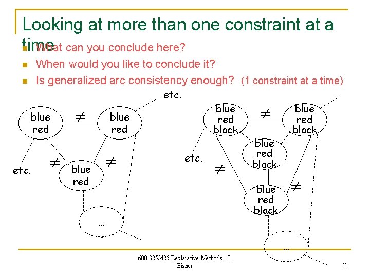
Looking at more than one constraint at a time n What can you conclude here? When would you like to conclude it? Is generalized arc consistency enough? (1 constraint at a time) n n etc. blue red etc. blue red black … blue red black … 600. 325/425 Declarative Methods - J. Eisner 41

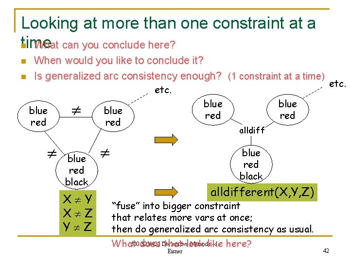
Looking at more than one constraint at a time n What can you conclude here? n n When would you like to conclude it? Is generalized arc consistency enough? (1 constraint at a time) etc. blue red black X Y X Z Y Z blue red alldiff blue red black alldifferent(X, Y, Z) “fuse” into bigger constraint that relates more vars at once; then do generalized arc consistency as usual. 600. 325/425 Methods - J. here? What does Declarative that look like Eisner 42 etc.

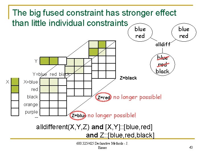
The big fused constraint has stronger effect than little individual constraints blue red alldiff blue red black Y Y=blue red black X Z=black X=blue red black Z=red no longer possible! orange purple … Z=blue no longer possible! alldifferent(X, Y, Z) and [X, Y]: : [blue, red] and Z: : [blue, red, black] 600. 325/425 Declarative Methods - J. Eisner 43

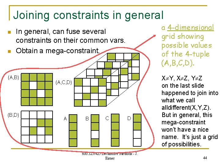
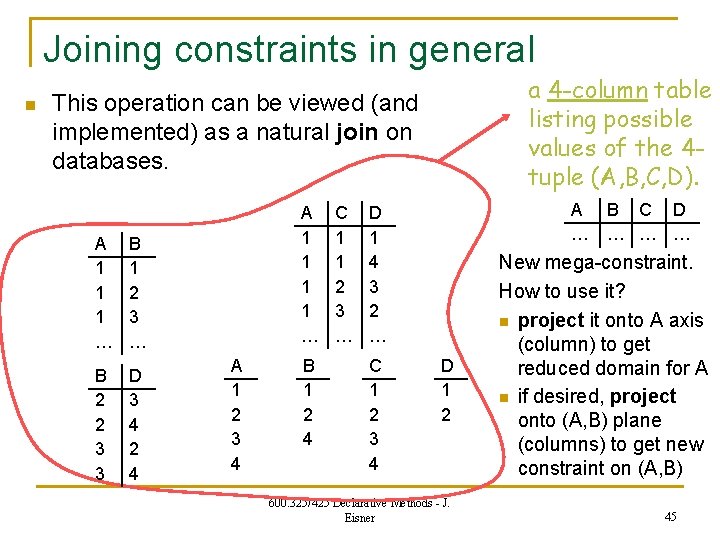
Joining constraints in general n n a 4 -dimensional grid showing possible values of the 4 -tuple (A, B, C, D). In general, can fuse several constraints on their common vars. Obtain a mega-constraint. (A, B) (B, D) (A, C, D) A B C D 600. 325/425 Declarative Methods - J. Eisner X Y, X Z, Y Z on the last slide happened to join into what we call alldifferent(X, Y, Z). But in general, this mega-constraint won’t have a nice name. It’s just a grid of possibilities. 44

Joining constraints in general n a 4 -column table listing possible values of the 4 tuple (A, B, C, D). This operation can be viewed (and implemented) as a natural join on databases. A 1 1 1 … B 1 2 3 … B 2 2 3 3 D 3 4 2 4 A 1 1 … A 1 2 3 4 B 1 2 4 C 1 1 2 3 … A … D 1 4 3 2 … C 1 2 3 4 D 1 2 600. 325/425 Declarative Methods - J. Eisner B C D … … … New mega-constraint. How to use it? n project it onto A axis (column) to get reduced domain for A n if desired, project onto (A, B) plane (columns) to get new constraint on (A, B) 45

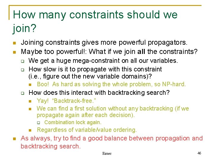
How many constraints should we join? n Joining constraints Which ones? gives more powerful propagators. n Maybe too powerful!: What if we join all the constraints? q q We get a huge mega-constraint on all our variables. How slow is it to propagate with this constraint (i. e. , figure out the new variable domains)? n q Boo! As hard as solving the whole problem, so NP-hard. How does this interact with backtracking search? n n Yay! “Backtrack-free. ” We can find a first solution without any backtracking (if we propagate again after each decision). q n n Combination lock again. Regardless of variable/value ordering. As always, try to find a good balance between propagation and backtracking search. 600. 325/425 Declarative Methods - J. Eisner 46

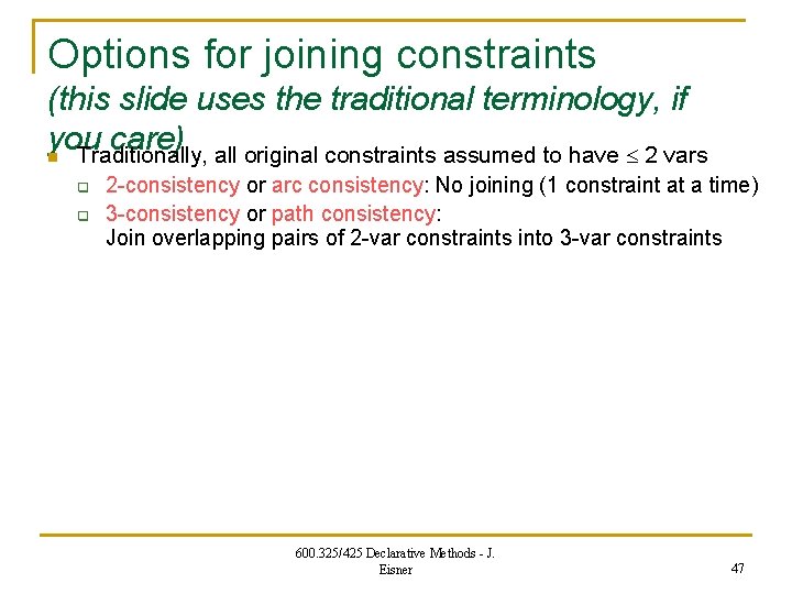
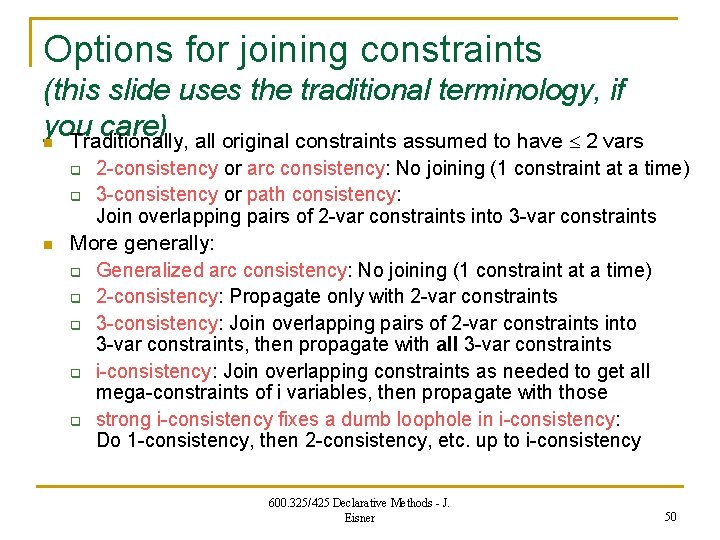
Options for joining constraints (this slide uses the traditional terminology, if you care) n Traditionally, all original constraints assumed to have 2 vars q q 2 -consistency or arc consistency: No joining (1 constraint at a time) 3 -consistency or path consistency: Join overlapping pairs of 2 -var constraints into 3 -var constraints 600. 325/425 Declarative Methods - J. Eisner 47

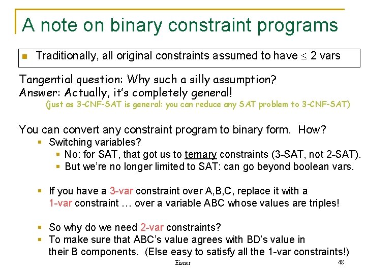
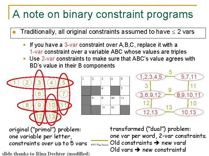
A note on binary constraint programs n Traditionally, all original constraints assumed to have 2 vars Tangential question: Why such a silly assumption? Answer: Actually, it’s completely general! (just as 3 -CNF-SAT is general: you can reduce any SAT problem to 3 -CNF-SAT) You can convert any constraint program to binary form. How? § Switching variables? § No: for SAT, that got us to ternary constraints (3 -SAT, not 2 -SAT). § But we’re no longer limited to SAT: can go beyond boolean vars. § If you have a 3 -var constraint over A, B, C, replace it with a 1 -var constraint … over a variable ABC whose values are triples! § So why do we need 2 -var constraints? § To make sure that ABC’s value agrees with BD’s value in their B components. 600. 325/425 (Else Declarative easy to. Methods satisfy - J. all the 1 -var constraints!) Eisner 48

A note on binary constraint programs n 1 Traditionally, all original constraints assumed to have 2 vars § If you have a 3 -var constraint over A, B, C, replace it with a 1 -var constraint over a variable ABC whose values are triples § Use 2 -var constraints to make sure that ABC’s value agrees with BD’s value in their B components 5 1, 2, 3, 4, 5 5, 7, 11 2 3 4 5 3 11 9 6 7 3, 6, 9, 12 8, 9, 10, 11 12 10 8 9 10 11 13 12, 13 10, 13 12 13 transformed (“dual”) problem: original (“primal”) problem: one var per word, 2 -var constraints. one variable per letter, Old constraints new vars! constraints over up to 5 vars 600. 325/425 Declarative Methods - J. 49 Eisner Old vars new constraints! slide thanks to Rina Dechter (modified)

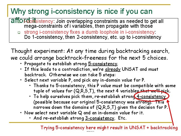
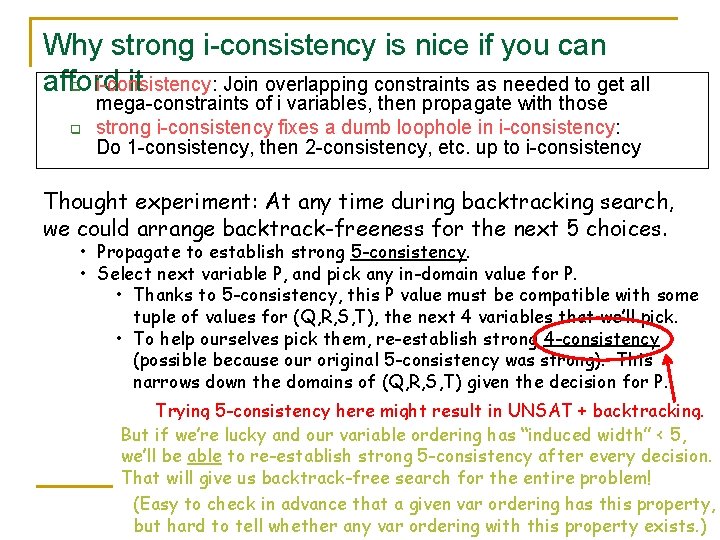
Options for joining constraints (this slide uses the traditional terminology, if you care) n Traditionally, all original constraints assumed to have 2 vars q q n 2 -consistency or arc consistency: No joining (1 constraint at a time) 3 -consistency or path consistency: Join overlapping pairs of 2 -var constraints into 3 -var constraints More generally: q Generalized arc consistency: No joining (1 constraint at a time) q 2 -consistency: Propagate only with 2 -var constraints q 3 -consistency: Join overlapping pairs of 2 -var constraints into 3 -var constraints, then propagate with all 3 -var constraints q i-consistency: Join overlapping constraints as needed to get all mega-constraints of i variables, then propagate with those q strong i-consistency fixes a dumb loophole in i-consistency: Do 1 -consistency, then 2 -consistency, etc. up to i-consistency 600. 325/425 Declarative Methods - J. Eisner 50

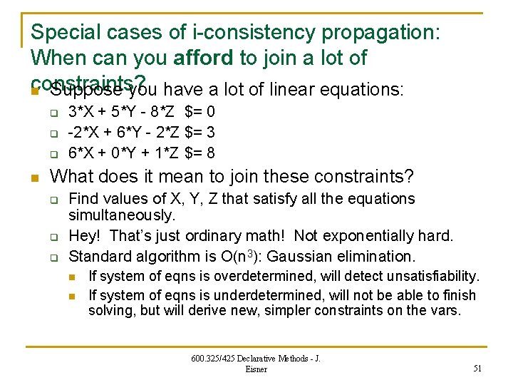
Special cases of i-consistency propagation: When can you afford to join a lot of constraints? n Suppose you have a lot of linear equations: q q q n 3*X + 5*Y - 8*Z $= 0 -2*X + 6*Y - 2*Z $= 3 6*X + 0*Y + 1*Z $= 8 What does it mean to join these constraints? q q q Find values of X, Y, Z that satisfy all the equations simultaneously. Hey! That’s just ordinary math! Not exponentially hard. Standard algorithm is O(n 3): Gaussian elimination. n n If system of eqns is overdetermined, will detect unsatisfiability. If system of eqns is underdetermined, will not be able to finish solving, but will derive new, simpler constraints on the vars. 600. 325/425 Declarative Methods - J. Eisner 51

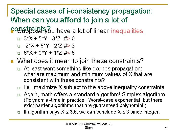
Special cases of i-consistency propagation: When can you afford to join a lot of constraints? n Suppose you have a lot of linear inequalities: q q q n 3*X + 5*Y - 8*Z #> 0 -2*X + 6*Y - 2*Z #> 3 6*X + 0*Y + 1*Z #< 8 What does it mean to join these constraints? q q At least want something like bounds propagation: what are maximum and minimum values of X that are consistent with these constraints? i. e. , maximize X subject to the above inequality constraints Again, math offers a standard algorithm! Simplex algorithm. (Polynomial-time in practice. Worst-case exponential, but there exist harder algorithms that are guaranteed polynomial. ) If algorithm says X 3. 6, we can conclude X 3 since integer. 600. 325/425 Declarative Methods - J. Eisner 52

Why strong i-consistency is nice if you can afford it q i-consistency: Join overlapping constraints as needed to get all q mega-constraints of i variables, then propagate with those strong i-consistency fixes a dumb loophole in i-consistency: Do 1 -consistency, then 2 -consistency, etc. up to i-consistency Thought experiment: At any time during backtracking search, we could arrange backtrack-freeness for the next 5 choices. • Propagate to establish strong 5 -consistency. • If this leads to a contradiction, we’re already UNSAT and must backtrack. Otherwise we can take 5 steps: • Select next variable P, and pick any in-domain value for P. • Thanks to 5 -consistency, this P value must be compatible with some tuple of values for (Q, R, S, T), the next 4 variables that we’ll pick. • To help ourselves pick them, re-establish strong 4 -consistency (possible because our original 5 -consistency was strong). This narrows down the domains of (Q, R, S, T) given the decision for P. • Now select next variable Q and an in-domain value for it. • And re-establish strong 3 -consistency. Etc. 600. 325/425 Declarative Methods -result J. Trying 5 -consistency here might in UNSAT + backtracking 53 Eisner

Why strong i-consistency is nice if you can afford it q i-consistency: Join overlapping constraints as needed to get all q mega-constraints of i variables, then propagate with those strong i-consistency fixes a dumb loophole in i-consistency: Do 1 -consistency, then 2 -consistency, etc. up to i-consistency Thought experiment: At any time during backtracking search, we could arrange backtrack-freeness for the next 5 choices. • Propagate to establish strong 5 -consistency. • Select next variable P, and pick any in-domain value for P. • Thanks to 5 -consistency, this P value must be compatible with some tuple of values for (Q, R, S, T), the next 4 variables that we’ll pick. • To help ourselves pick them, re-establish strong 4 -consistency (possible because our original 5 -consistency was strong). This narrows down the domains of (Q, R, S, T) given the decision for P. Trying 5 -consistency here might result in UNSAT + backtracking. But if we’re lucky and our variable ordering has “induced width” < 5, we’ll be able to re-establish strong 5 -consistency after every decision. That will give us backtrack-free search for the entire problem! Declarative - J. var ordering has this property, (Easy to check in 600. 325/425 advance that Methods a given 54 Eisner but hard to tell whether any var ordering with this property exists. )

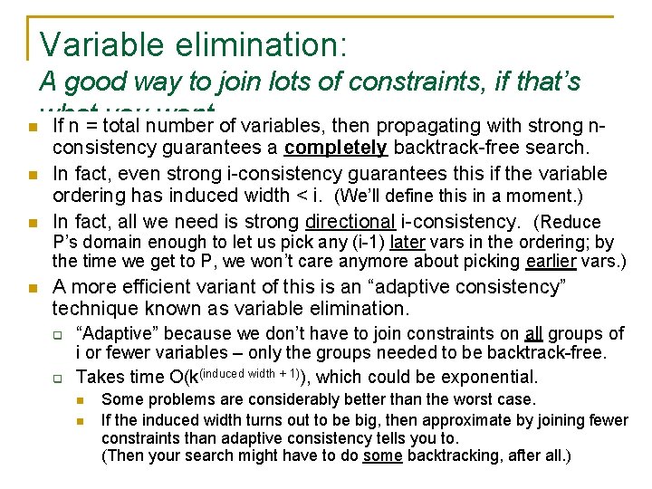
Variable elimination: A good way to join lots of constraints, if that’s what you want n If n = total number of variables, then propagating with strong nn n consistency guarantees a completely backtrack-free search. In fact, even strong i-consistency guarantees this if the variable ordering has induced width < i. (We’ll define this in a moment. ) In fact, all we need is strong directional i-consistency. (Reduce P’s domain enough to let us pick any (i-1) later vars in the ordering; by the time we get to P, we won’t care anymore about picking earlier vars. ) n A more efficient variant of this is an “adaptive consistency” technique known as variable elimination. q q “Adaptive” because we don’t have to join constraints on all groups of i or fewer variables – only the groups needed to be backtrack-free. Takes time O(k(induced width + 1)), which could be exponential. n n Some problems are considerably better than the worst case. If the induced width turns out to be big, then approximate by joining fewer constraints than adaptive consistency tells you to. 600. 325/425 Declarative - J. backtracking, after all. ) (Then your search might have to do. Methods some Eisner 55

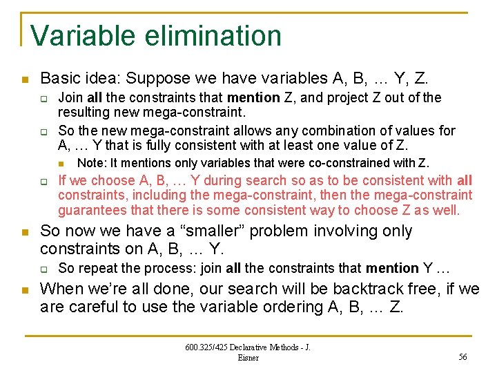
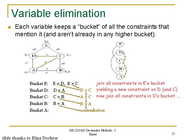
Variable elimination n Basic idea: Suppose we have variables A, B, … Y, Z. q q Join all the constraints that mention Z, and project Z out of the resulting new mega-constraint. So the new mega-constraint allows any combination of values for A, … Y that is fully consistent with at least one value of Z. n q n If we choose A, B, … Y during search so as to be consistent with all constraints, including the mega-constraint, then the mega-constraint guarantees that there is some consistent way to choose Z as well. So now we have a “smaller” problem involving only constraints on A, B, … Y. q n Note: It mentions only variables that were co-constrained with Z. So repeat the process: join all the constraints that mention Y … When we’re all done, our search will be backtrack free, if we are careful to use the variable ordering A, B, … Z. 600. 325/425 Declarative Methods - J. Eisner 56

Variable elimination n Each variable keeps a “bucket” of all the constraints that mention it (and aren’t already in any higher bucket). = = Bucket E: E D, E C Bucket D: D A Bucket C: C B Bucket B: B A Bucket A: slide thanks to Rina Dechter join all constraints in E’s bucket yielding a new constraint on D (and C) now join all constraints in D’s bucket … D=C A C B=A contradiction 600. 325/425 Declarative Methods - J. Eisner 57

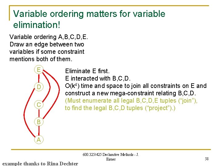
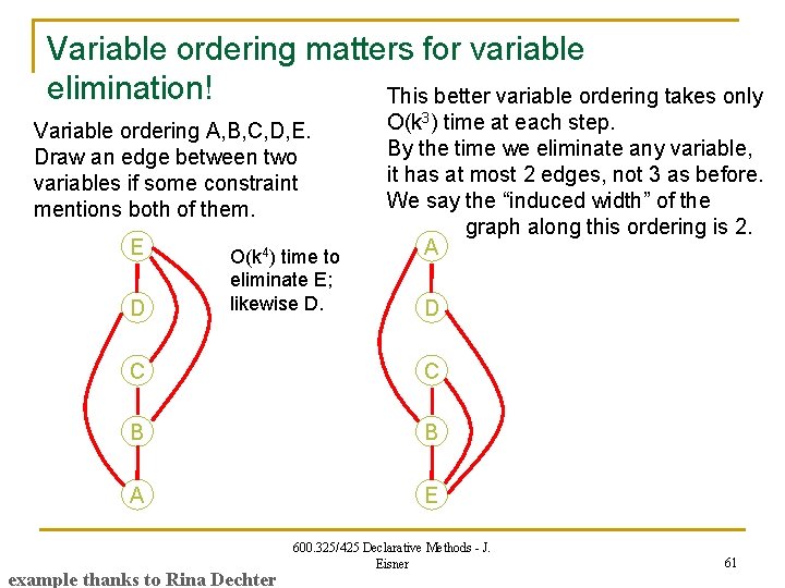
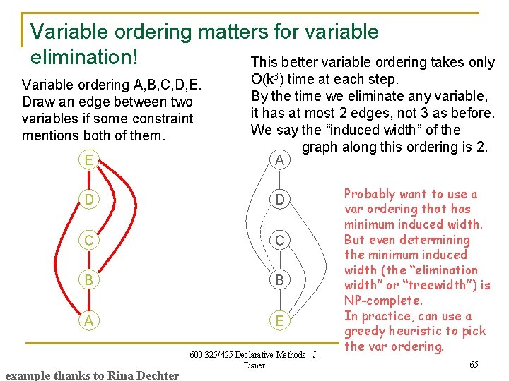
Variable ordering matters for variable elimination! Variable ordering A, B, C, D, E. Draw an edge between two variables if some constraint mentions both of them. E D C Eliminate E first. E interacted with B, C, D. O(k 4) time and space to join all constraints on E and construct a new mega-constraint relating B, C, D. (Must enumerate all legal B, C, D, E tuples (“join”), to find the legal B, C, D tuples (“project”). ) B A example thanks to Rina Dechter 600. 325/425 Declarative Methods - J. Eisner 58

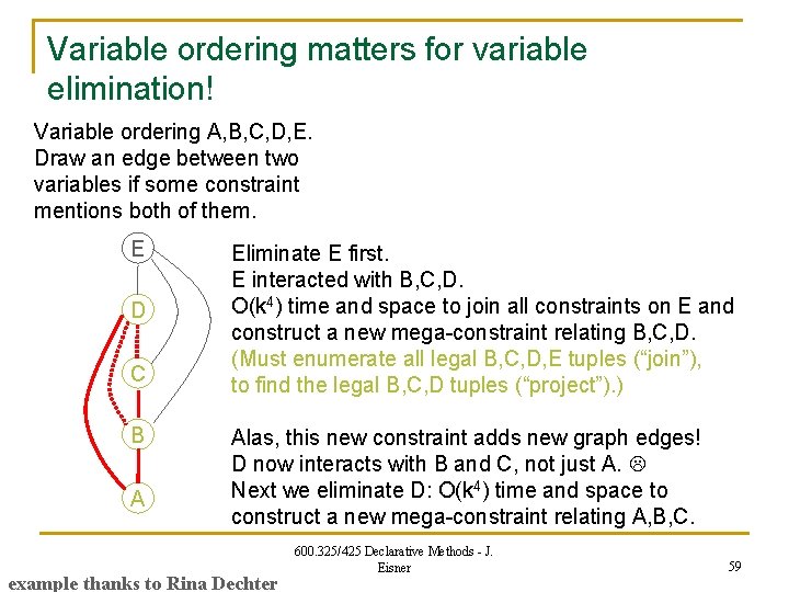
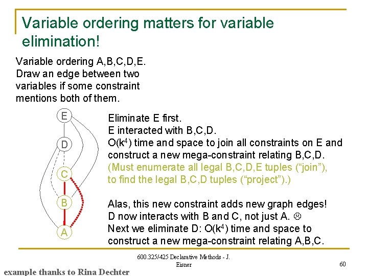
Variable ordering matters for variable elimination! Variable ordering A, B, C, D, E. Draw an edge between two variables if some constraint mentions both of them. E D C B A Eliminate E first. E interacted with B, C, D. O(k 4) time and space to join all constraints on E and construct a new mega-constraint relating B, C, D. (Must enumerate all legal B, C, D, E tuples (“join”), to find the legal B, C, D tuples (“project”). ) Alas, this new constraint adds new graph edges! D now interacts with B and C, not just A. Next we eliminate D: O(k 4) time and space to construct a new mega-constraint relating A, B, C. example thanks to Rina Dechter 600. 325/425 Declarative Methods - J. Eisner 59

Variable ordering matters for variable elimination! Variable ordering A, B, C, D, E. Draw an edge between two variables if some constraint mentions both of them. E D C B A Eliminate E first. E interacted with B, C, D. O(k 4) time and space to join all constraints on E and construct a new mega-constraint relating B, C, D. (Must enumerate all legal B, C, D, E tuples (“join”), to find the legal B, C, D tuples (“project”). ) Alas, this new constraint adds new graph edges! D now interacts with B and C, not just A. Next we eliminate D: O(k 4) time and space to construct a new mega-constraint relating A, B, C. example thanks to Rina Dechter 600. 325/425 Declarative Methods - J. Eisner 60

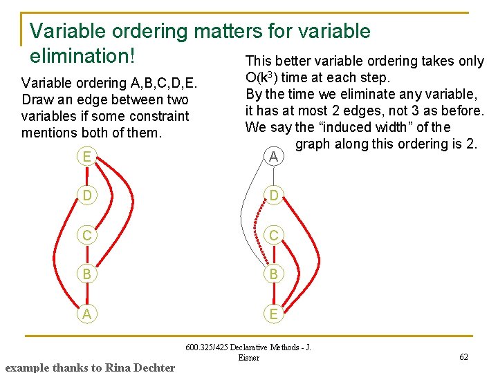
Variable ordering matters for variable elimination! This better variable ordering takes only Variable ordering A, B, C, D, E. Draw an edge between two variables if some constraint mentions both of them. E D O(k 4) time to eliminate E; likewise D. O(k 3) time at each step. By the time we eliminate any variable, it has at most 2 edges, not 3 as before. We say the “induced width” of the graph along this ordering is 2. A D C C B B A E example thanks to Rina Dechter 600. 325/425 Declarative Methods - J. Eisner 61

Variable ordering matters for variable elimination! This better variable ordering takes only Variable ordering A, B, C, D, E. Draw an edge between two variables if some constraint mentions both of them. E O(k 3) time at each step. By the time we eliminate any variable, it has at most 2 edges, not 3 as before. We say the “induced width” of the graph along this ordering is 2. A D D C C B B A E example thanks to Rina Dechter 600. 325/425 Declarative Methods - J. Eisner 62

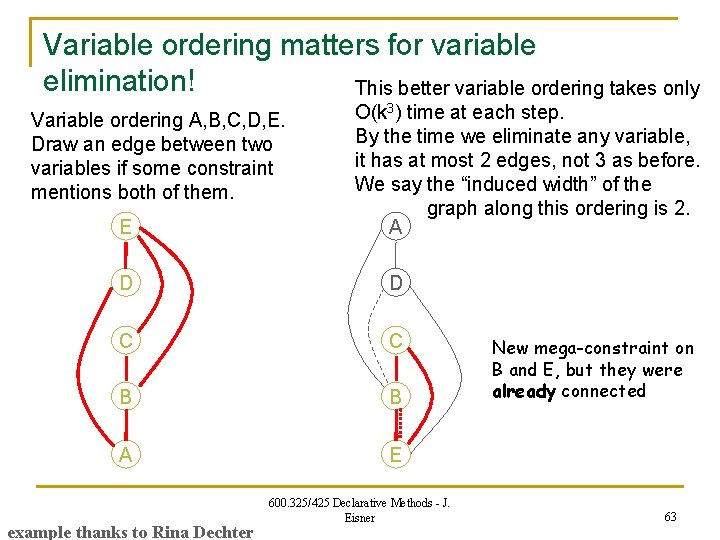
Variable ordering matters for variable elimination! This better variable ordering takes only Variable ordering A, B, C, D, E. Draw an edge between two variables if some constraint mentions both of them. E O(k 3) time at each step. By the time we eliminate any variable, it has at most 2 edges, not 3 as before. We say the “induced width” of the graph along this ordering is 2. A D D C C B B A E example thanks to Rina Dechter 600. 325/425 Declarative Methods - J. Eisner New mega-constraint on B and E, but they were already connected 63

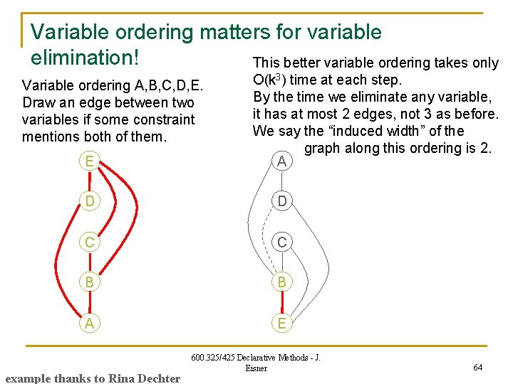
Variable ordering matters for variable elimination! This better variable ordering takes only Variable ordering A, B, C, D, E. Draw an edge between two variables if some constraint mentions both of them. E O(k 3) time at each step. By the time we eliminate any variable, it has at most 2 edges, not 3 as before. We say the “induced width” of the graph along this ordering is 2. A D D C C B B A E example thanks to Rina Dechter 600. 325/425 Declarative Methods - J. Eisner 64

Variable ordering matters for variable elimination! This better variable ordering takes only Variable ordering A, B, C, D, E. Draw an edge between two variables if some constraint mentions both of them. E O(k 3) time at each step. By the time we eliminate any variable, it has at most 2 edges, not 3 as before. We say the “induced width” of the graph along this ordering is 2. A D D C C B B A E example thanks to Rina Dechter 600. 325/425 Declarative Methods - J. Eisner Probably want to use a var ordering that has minimum induced width. But even determining the minimum induced width (the “elimination width” or “treewidth”) is NP-complete. In practice, can use a greedy heuristic to pick the var ordering. 65

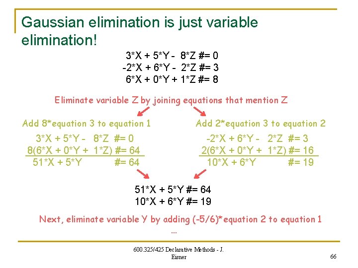
Gaussian elimination is just variable elimination! 3*X + 5*Y - 8*Z #= 0 -2*X + 6*Y - 2*Z #= 3 6*X + 0*Y + 1*Z #= 8 Eliminate variable Z by joining equations that mention Z Add 8*equation 3 to equation 1 3*X + 5*Y - 8*Z #= 0 8(6*X + 0*Y + 1*Z) #= 64 51*X + 5*Y #= 64 Add 2*equation 3 to equation 2 -2*X + 6*Y - 2*Z #= 3 2(6*X + 0*Y + 1*Z) #= 16 10*X + 6*Y #= 19 51*X + 5*Y #= 64 10*X + 6*Y #= 19 Next, eliminate variable Y by adding (-5/6)*equation 2 to equation 1 … 600. 325/425 Declarative Methods - J. Eisner 66

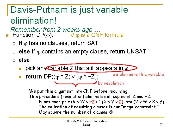
Davis-Putnam is just variable elimination! Remember from 2 weeks ago … n Function DP( ): // is a CNF formula q if has no clauses, return SAT q else if contains an empty clause, return UNSAT q else n pick any variable Z that still appears in we eliminate this variable n return DP(( ^ Z) v ( ^ ~Z)) by resolution We put this argument into CNF before recursing This procedure (resolution) eliminates all copies of Z and ~Z. Fuses each pair (V v W v ~Z) ^ (X v Y v Z) into (V v W v X v Y) The collection of resulting clauses is our “mega-constraint. ” May square the number of clauses 600. 325/425 Declarative Methods - J. Eisner 67

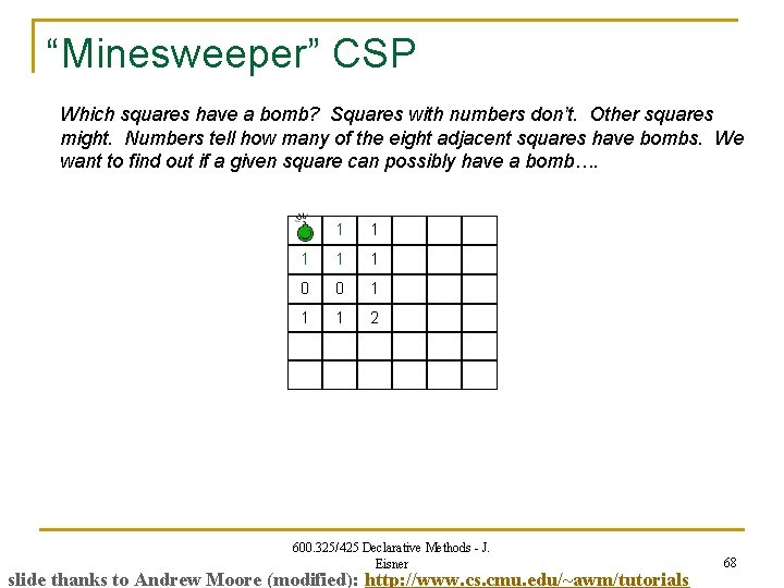
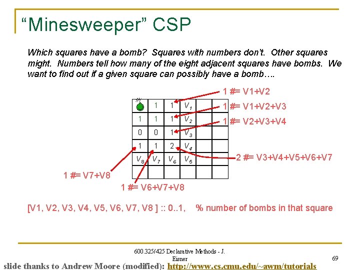
“Minesweeper” CSP Which squares have a bomb? Squares with numbers don’t. Other squares might. Numbers tell how many of the eight adjacent squares have bombs. We want to find out if a given square can possibly have a bomb…. 1 1 1 0 0 1 1 1 2 600. 325/425 Declarative Methods - J. Eisner slide thanks to Andrew Moore (modified): http: //www. cs. cmu. edu/~awm/tutorials 68

“Minesweeper” CSP Which squares have a bomb? Squares with numbers don’t. Other squares might. Numbers tell how many of the eight adjacent squares have bombs. We want to find out if a given square can possibly have a bomb…. 1 #= V 1+V 2 1 1 V 1 1 #= V 1+V 2+V 3 1 1 1 V 2 1 #= V 2+V 3+V 4 0 0 1 V 3 1 1 2 V 4 V 8 V 7 V 6 V 5 2 #= V 3+V 4+V 5+V 6+V 7 1 #= V 7+V 8 1 #= V 6+V 7+V 8 [V 1, V 2, V 3, V 4, V 5, V 6, V 7, V 8 ] : : 0. . 1, % number of bombs in that square 600. 325/425 Declarative Methods - J. Eisner slide thanks to Andrew Moore (modified): http: //www. cs. cmu. edu/~awm/tutorials 69

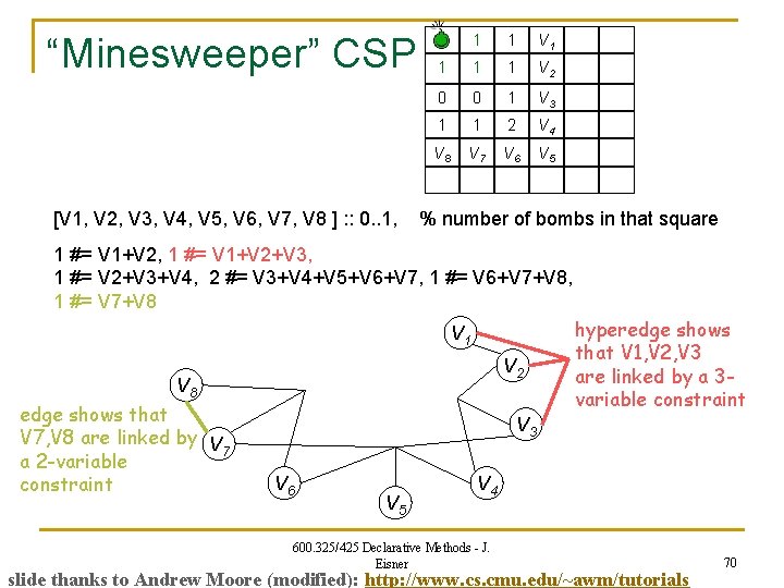
“Minesweeper” CSP [V 1, V 2, V 3, V 4, V 5, V 6, V 7, V 8 ] : : 0. . 1, 1 1 V 2 0 0 1 V 3 1 1 2 V 4 V 8 V 7 V 6 V 5 % number of bombs in that square 1 #= V 1+V 2, 1 #= V 1+V 2+V 3, 1 #= V 2+V 3+V 4, 2 #= V 3+V 4+V 5+V 6+V 7, 1 #= V 6+V 7+V 8, 1 #= V 7+V 8 V 1 V 2 V 8 edge shows that V 7, V 8 are linked by V 7 a 2 -variable constraint hyperedge shows that V 1, V 2, V 3 are linked by a 3 variable constraint V 3 V 6 V 5 V 4 600. 325/425 Declarative Methods - J. Eisner slide thanks to Andrew Moore (modified): http: //www. cs. cmu. edu/~awm/tutorials 70

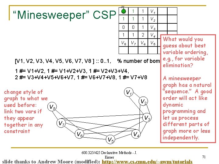
“Minesweeper” CSP 1 1 V 2 0 0 1 V 3 1 1 2 V 4 V 8 V 7 V 6 V 5 What would you guess about best variable ordering, e. g. , for square variable [V 1, V 2, V 3, V 4, V 5, V 6, V 7, V 8 ] : : 0. . 1, % number of bombs in that elimination? 1 #= V 1+V 2, 1 #= V 1+V 2+V 3, 1 #= V 2+V 3+V 4, 2 #= V 3+V 4+V 5+V 6+V 7, 1 #= V 6+V 7+V 8, 1 #= V 7+V 8 A minesweeper graph has a natural “sequence. ” A good change style of V 1 order will act like graph to what we V 2 dynamic used before: V 8 programming and link two vars if V 3 let us process they appear V 7 different parts of together in any graph more or less constraint V 6 V 4 independently. V 5 600. 325/425 Declarative Methods - J. Eisner slide thanks to Andrew Moore (modified): http: //www. cs. cmu. edu/~awm/tutorials 71

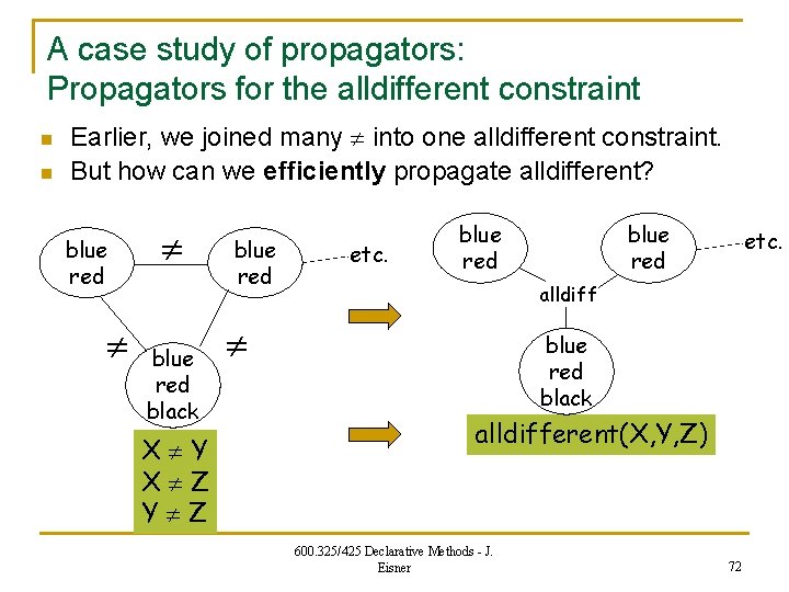
A case study of propagators: Propagators for the alldifferent constraint n n Earlier, we joined many into one alldifferent constraint. But how can we efficiently propagate alldifferent? blue red black X Y X Z Y Z blue red etc. alldiff blue red black alldifferent(X, Y, Z) 600. 325/425 Declarative Methods - J. Eisner 72

A case study: Propagators for the alldifferent constraint n n Earlier, we joined many into one alldifferent constraint. But how can we efficiently propagate alldifferent? Often it’s useful to write alldifferent(a whole bunch of vars). Option 1: Treat it like a collection of pairwise So if we learn that X=3, eliminate 3 from domains of Y, Z, … No propagation if we learn that X: : [3, 4]. Must narrow X down to a single value in order to propagate. 600. 325/425 Declarative Methods - J. Eisner 73

A case study: Propagators for the alldifferent constraint n n Earlier, we joined many into one alldifferent constraint. But how can we efficiently propagate alldifferent? Often it’s useful to write alldifferent(a whole bunch of vars). Option 2: Just like option 1 (a collection of pairwise ), but add the “pigeonhole principle. ” That is, do a quick check for unsatisfiability: for alldifferent(A, B, …J) over 10 variables, be sure to fail if the union of their domains becomes smaller than 10 values. That failure will force backtracking. 600. 325/425 Declarative Methods - J. Eisner 74

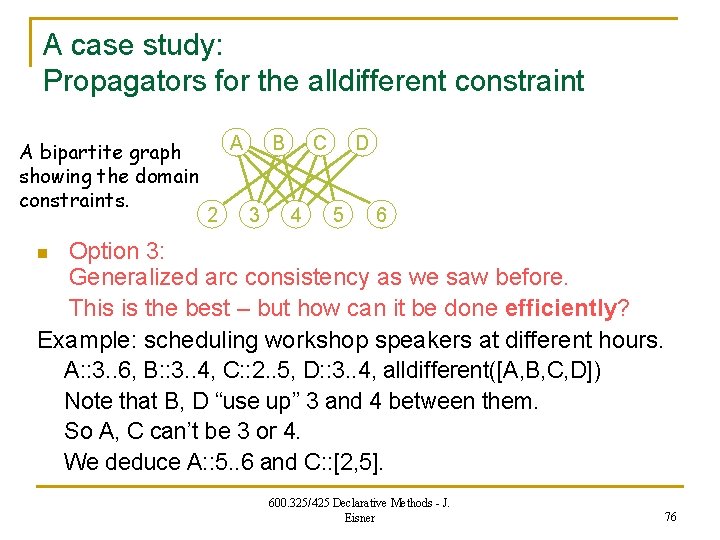
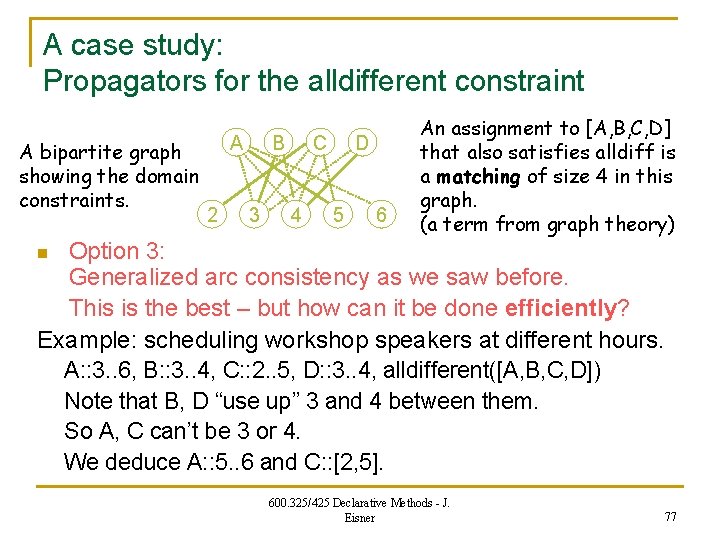
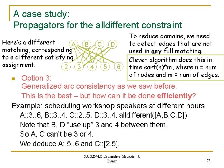
A case study: Propagators for the alldifferent constraint n n Earlier, we joined many into one alldifferent constraint. But how can we efficiently propagate alldifferent? Often it’s useful to write alldifferent(a whole bunch of vars). Option 3: Generalized arc consistency as we saw before. Example: scheduling workshop speakers at different hours. A: : 3. . 6, B: : 3. . 4, C: : 2. . 5, D: : 3. . 4, alldifferent([A, B, C, D]) Note that B, D “use up” 3 and 4 between them. So A, C can’t be 3 or 4. We deduce A: : 5. . 6 and C: : [2, 5]. 600. 325/425 Declarative Methods - J. Eisner 75

A case study: Propagators for the alldifferent constraint A bipartite graph showing the domain constraints. A 2 B 3 C 4 D 5 6 Option 3: Generalized arc consistency as we saw before. This is the best – but how can it be done efficiently? Example: scheduling workshop speakers at different hours. A: : 3. . 6, B: : 3. . 4, C: : 2. . 5, D: : 3. . 4, alldifferent([A, B, C, D]) Note that B, D “use up” 3 and 4 between them. So A, C can’t be 3 or 4. We deduce A: : 5. . 6 and C: : [2, 5]. n 600. 325/425 Declarative Methods - J. Eisner 76

A case study: Propagators for the alldifferent constraint A bipartite graph showing the domain constraints. A 2 B 3 C 4 D 5 6 An assignment to [A, B, C, D] that also satisfies alldiff is a matching of size 4 in this graph. (a term from graph theory) Option 3: Generalized arc consistency as we saw before. This is the best – but how can it be done efficiently? Example: scheduling workshop speakers at different hours. A: : 3. . 6, B: : 3. . 4, C: : 2. . 5, D: : 3. . 4, alldifferent([A, B, C, D]) Note that B, D “use up” 3 and 4 between them. So A, C can’t be 3 or 4. We deduce A: : 5. . 6 and C: : [2, 5]. n 600. 325/425 Declarative Methods - J. Eisner 77

A case study: Propagators for the alldifferent constraint Here’s a different A B C D matching, corresponding to a different satisfying assignment. 2 3 4 5 6 To reduce domains, we need to detect edges that are not used in any full matching. Clever algorithm does this in time sqrt(n)*m, where n = num of nodes and m = num of edges. Option 3: Generalized arc consistency as we saw before. This is the best – but how can it be done efficiently? Example: scheduling workshop speakers at different hours. A: : 3. . 6, B: : 3. . 4, C: : 2. . 5, D: : 3. . 4, alldifferent([A, B, C, D]) Note that B, D “use up” 3 and 4 between them. So A, C can’t be 3 or 4. We deduce A: : 5. . 6 and C: : [2, 5]. n 600. 325/425 Declarative Methods - J. Eisner 78

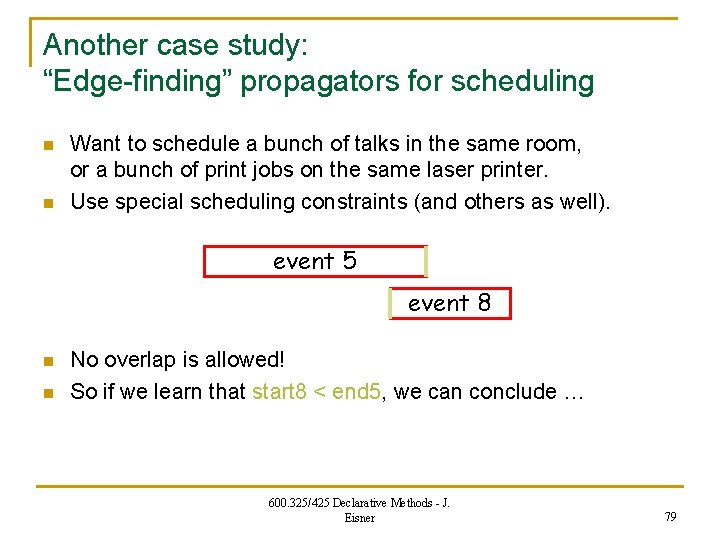
Another case study: “Edge-finding” propagators for scheduling n n Want to schedule a bunch of talks in the same room, or a bunch of print jobs on the same laser printer. Use special scheduling constraints (and others as well). event 5 event 8 n n No overlap is allowed! So if we learn that start 8 < end 5, we can conclude … 600. 325/425 Declarative Methods - J. Eisner 79

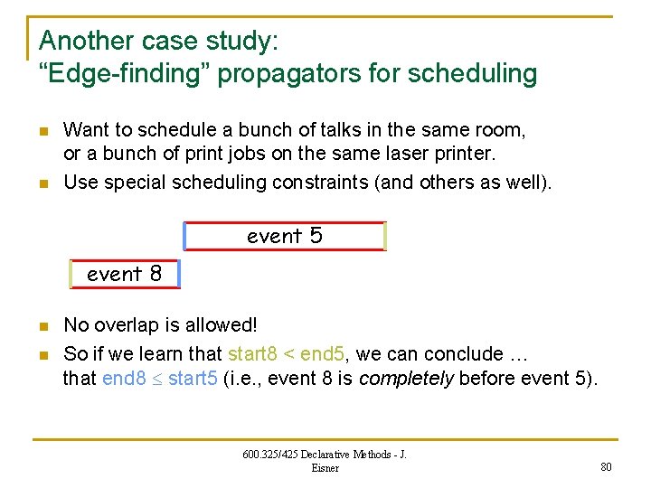
Another case study: “Edge-finding” propagators for scheduling n n Want to schedule a bunch of talks in the same room, or a bunch of print jobs on the same laser printer. Use special scheduling constraints (and others as well). event 5 event 8 n n No overlap is allowed! So if we learn that start 8 < end 5, we can conclude … that end 8 start 5 (i. e. , event 8 is completely before event 5). 600. 325/425 Declarative Methods - J. Eisner 80

One more idea: Relaxation (a third major technique, alongside propagation and search) n n n Suppose you have a huge collection of constraints – maybe exponentially many – too many to use all at once. Ignore some of them, giving a “relaxed” problem. Solve that first: q If you were lucky, solution satisfies most of the ignored constraints too. q Add in any few of the constraints that were violated and try again. The new constraints “cut off” the solution you just found. That’s how traveling salesperson problems are solved! q q n http: //www. tsp. gatech. edu/methods/dfj - clear explanation http: //www. tsp. gatech. edu/methods/cpapp - interactive Java applet Common to relax constraints saying that some vars must be integers: q Then you can use traditional fast equation solvers for real numbers. q If you get fractional solutions, add new linear constraints (“cutting planes”) to cut those off. q In particular, integer linear programming (ILP) is NP-complete – and many problems can naturally be reduced to ILP and solved by an ILP solver. 600. 325/425 Declarative Methods - J. Eisner 81

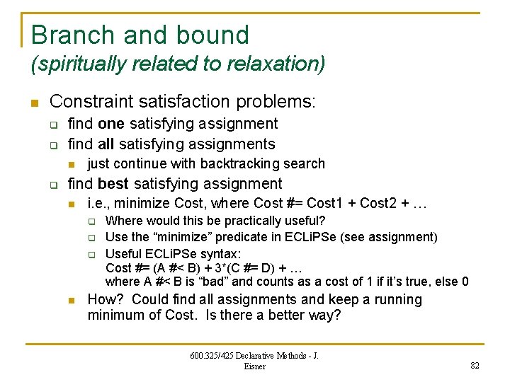
Branch and bound (spiritually related to relaxation) n Constraint satisfaction problems: q q find one satisfying assignment find all satisfying assignments n q just continue with backtracking search find best satisfying assignment n i. e. , minimize Cost, where Cost #= Cost 1 + Cost 2 + … q q q n Where would this be practically useful? Use the “minimize” predicate in ECLi. PSe (see assignment) Useful ECLi. PSe syntax: Cost #= (A #< B) + 3*(C #= D) + … where A #< B is “bad” and counts as a cost of 1 if it’s true, else 0 How? Could find all assignments and keep a running minimum of Cost. Is there a better way? 600. 325/425 Declarative Methods - J. Eisner 82

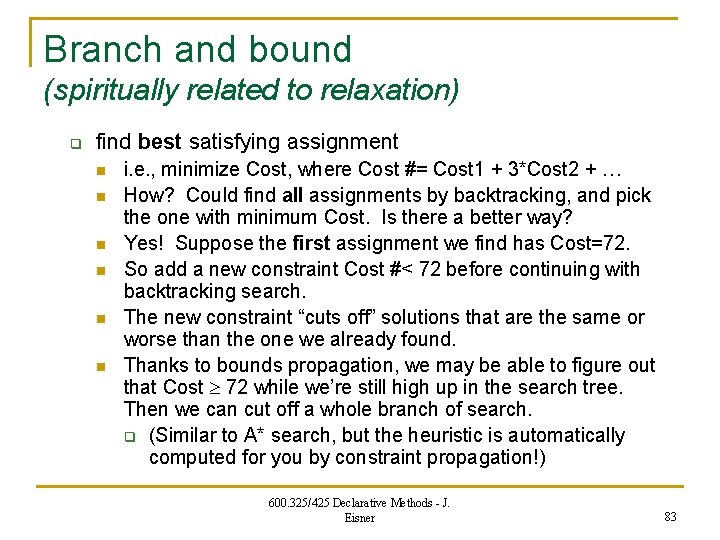
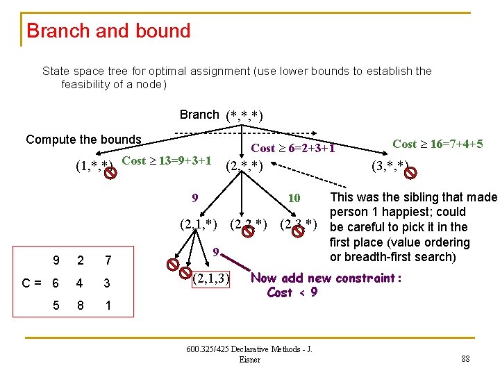
Branch and bound (spiritually related to relaxation) q find best satisfying assignment n n n i. e. , minimize Cost, where Cost #= Cost 1 + 3*Cost 2 + … How? Could find all assignments by backtracking, and pick the one with minimum Cost. Is there a better way? Yes! Suppose the first assignment we find has Cost=72. So add a new constraint Cost #< 72 before continuing with backtracking search. The new constraint “cuts off” solutions that are the same or worse than the one we already found. Thanks to bounds propagation, we may be able to figure out that Cost 72 while we’re still high up in the search tree. Then we can cut off a whole branch of search. q (Similar to A* search, but the heuristic is automatically computed for you by constraint propagation!) 600. 325/425 Declarative Methods - J. Eisner 83

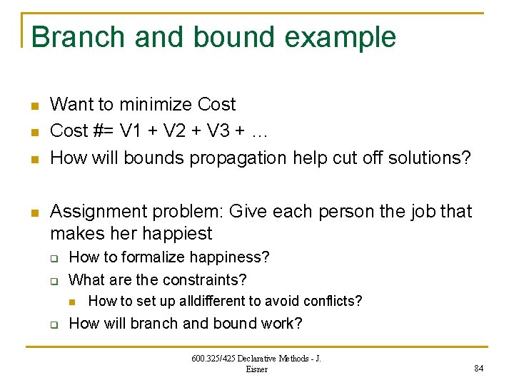
Branch and bound example n n Want to minimize Cost #= V 1 + V 2 + V 3 + … How will bounds propagation help cut off solutions? Assignment problem: Give each person the job that makes her happiest q q How to formalize happiness? What are the constraints? n q How to set up alldifferent to avoid conflicts? How will branch and bound work? 600. 325/425 Declarative Methods - J. Eisner 84

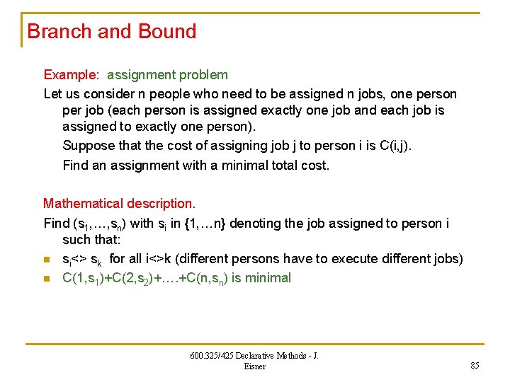
Branch and Bound Example: assignment problem Let us consider n people who need to be assigned n jobs, one person per job (each person is assigned exactly one job and each job is assigned to exactly one person). Suppose that the cost of assigning job j to person i is C(i, j). Find an assignment with a minimal total cost. Mathematical description. Find (s 1, …, sn) with si in {1, …n} denoting the job assigned to person i such that: n si<> sk for all i<>k (different persons have to execute different jobs) n C(1, s 1)+C(2, s 2)+…. +C(n, sn) is minimal 600. 325/425 Declarative Methods - J. Eisner 85

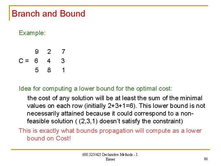
Branch and Bound Example: 9 C= 6 5 2 4 8 7 3 1 Idea for computing a lower bound for the optimal cost: the cost of any solution will be at least the sum of the minimal values on each row (initially 2+3+1=6). This lower bound is not necessarily attained because it could correspond to a nonfeasible solution ( (2, 3, 1) doesn’t satisfy the constraint) This is exactly what bounds propagation will compute as a lower bound on Cost! 600. 325/425 Declarative Methods - J. Eisner 86

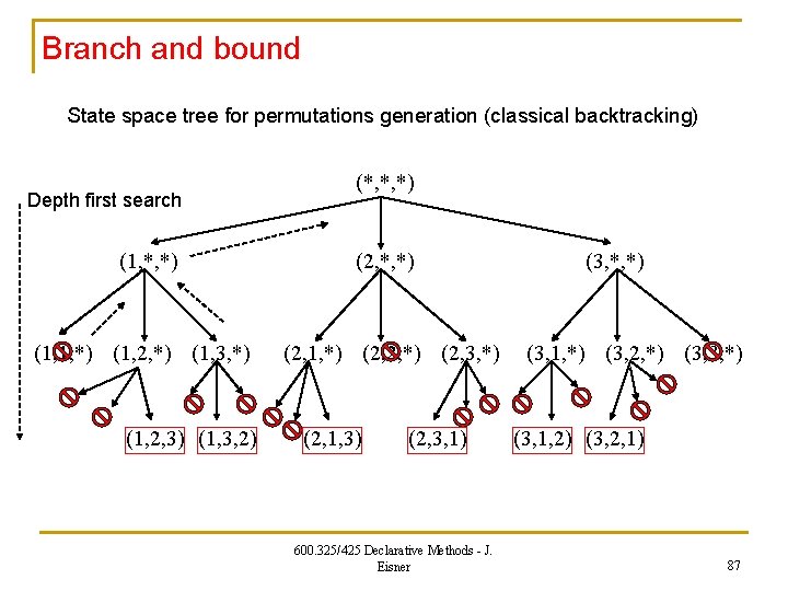
Branch and bound State space tree for permutations generation (classical backtracking) Depth first search (*, *, *) (1, *, *) (2, *, *) (1, 1, *) (1, 2, *) (1, 3, *) (2, 1, *) (2, 2, *) (2, 3, *) (1, 2, 3) (1, 3, 2) (2, 1, 3) (2, 3, 1) 600. 325/425 Declarative Methods - J. Eisner (3, *, *) (3, 1, *) (3, 2, *) (3, 3, *) (3, 1, 2) (3, 2, 1) 87

Branch and bound State space tree for optimal assignment (use lower bounds to establish the feasibility of a node) Branch (*, *, *) Compute the bounds Cost 6=2+3+1 (1, *, *) Cost 13=9+3+1 (2, *, *) 9 (3, *, *) 10 (2, 1, *) (2, 2, *) (2, 3, *) 9 2 7 C= 6 4 3 5 8 1 9 (2, 1, 3) Cost 16=7+4+5 This was the sibling that made person 1 happiest; could be careful to pick it in the first place (value ordering or breadth-first search) Now add new constraint: Cost < 9 600. 325/425 Declarative Methods - J. Eisner 88