CS 188 Artificial Intelligence Constraint Satisfaction Problems II

CS 188: Artificial Intelligence Constraint Satisfaction Problems II and Local Search Instructors: Sergey Levine and Stuart Russell University of California, Berkeley [These slides were created by Dan Klein and Pieter Abbeel for CS 188 Intro to AI at UC Berkeley. All CS 188 materials are available at http: //ai. berkeley. edu. ]

Today § Structure of CSPs § Local Search

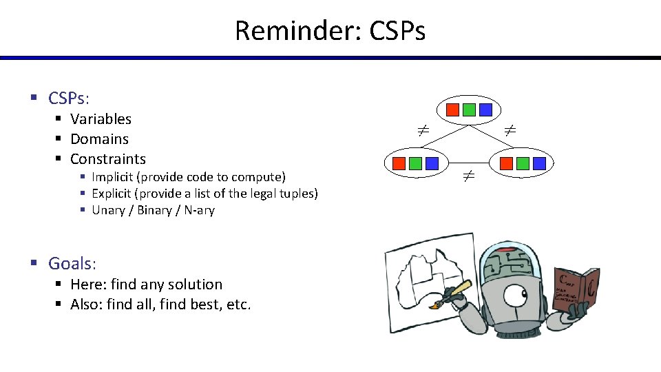
Reminder: CSPs § CSPs: § Variables § Domains § Constraints § Implicit (provide code to compute) § Explicit (provide a list of the legal tuples) § Unary / Binary / N-ary § Goals: § Here: find any solution § Also: find all, find best, etc.

Standard Search Problems § Standard search problems: § § State is a black box: arbitrary data structure Goal test is a black box test on states Actions are black box data structures Transition model is a black box function § Consequences: § Have to write new code for every new problem § Have to devise heuristics for each new problem § Cannot just choose actions that achieve the goal! § Solution: formal representation for states, actions, goals

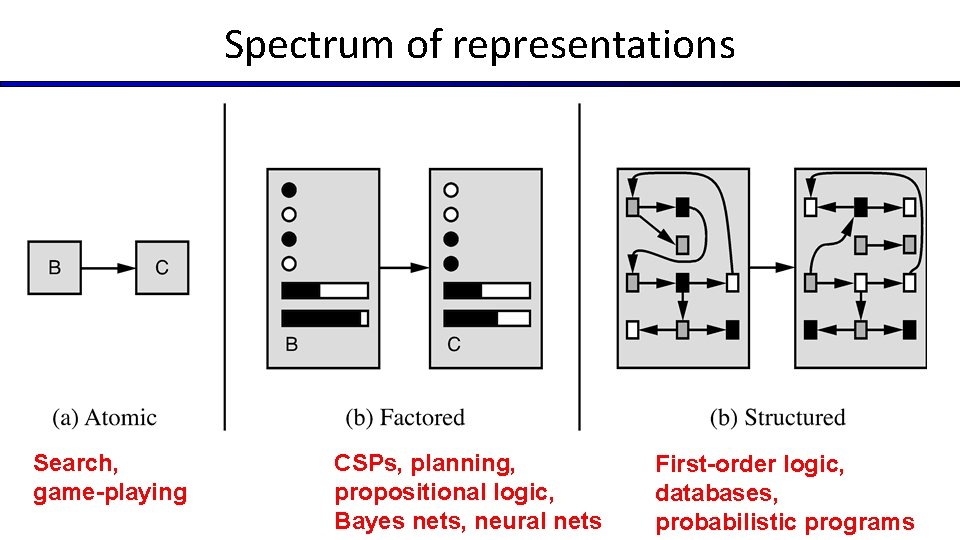
Spectrum of representations Search, game-playing CSPs, planning, propositional logic, Bayes nets, neural nets First-order logic, databases, probabilistic programs

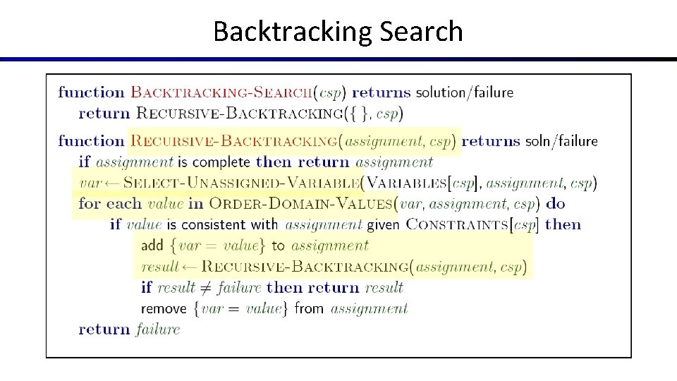
Backtracking Search

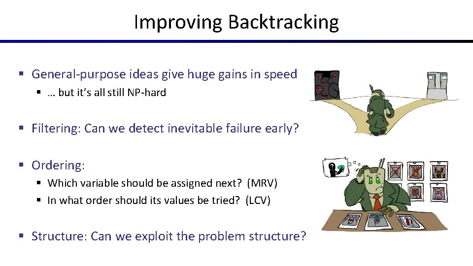
Improving Backtracking § General-purpose ideas give huge gains in speed § … but it’s all still NP-hard § Filtering: Can we detect inevitable failure early? § Ordering: § Which variable should be assigned next? (MRV) § In what order should its values be tried? (LCV) § Structure: Can we exploit the problem structure?

Structure

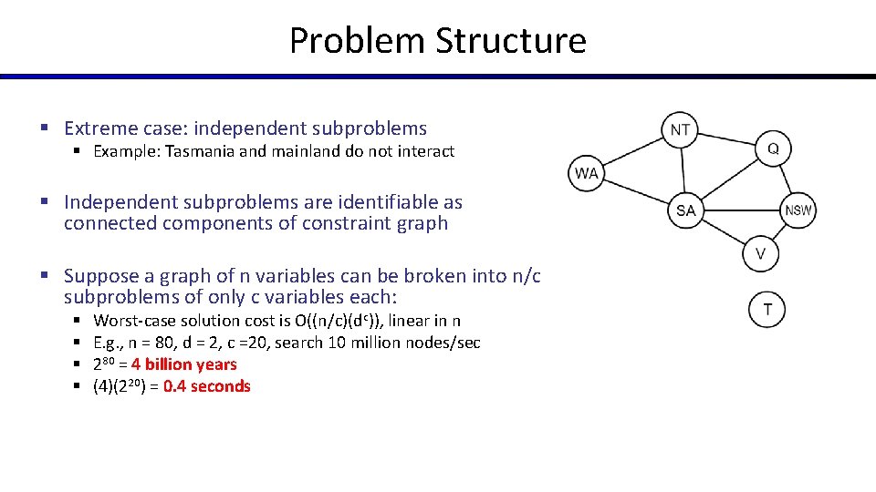
Problem Structure § Extreme case: independent subproblems § Example: Tasmania and mainland do not interact § Independent subproblems are identifiable as connected components of constraint graph § Suppose a graph of n variables can be broken into n/c subproblems of only c variables each: § § Worst-case solution cost is O((n/c)(dc)), linear in n E. g. , n = 80, d = 2, c =20, search 10 million nodes/sec 280 = 4 billion years (4)(220) = 0. 4 seconds

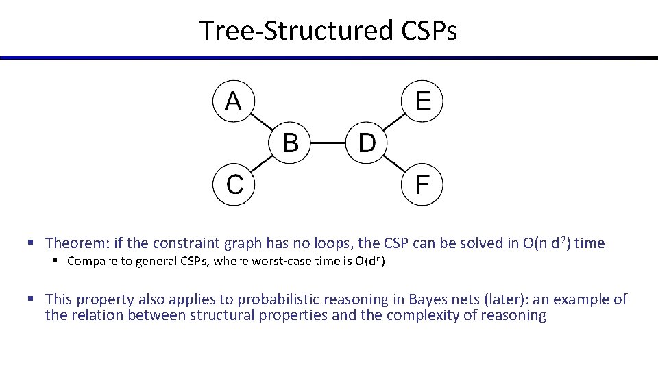
Tree-Structured CSPs § Theorem: if the constraint graph has no loops, the CSP can be solved in O(n d 2) time § Compare to general CSPs, where worst-case time is O(dn) § This property also applies to probabilistic reasoning in Bayes nets (later): an example of the relation between structural properties and the complexity of reasoning

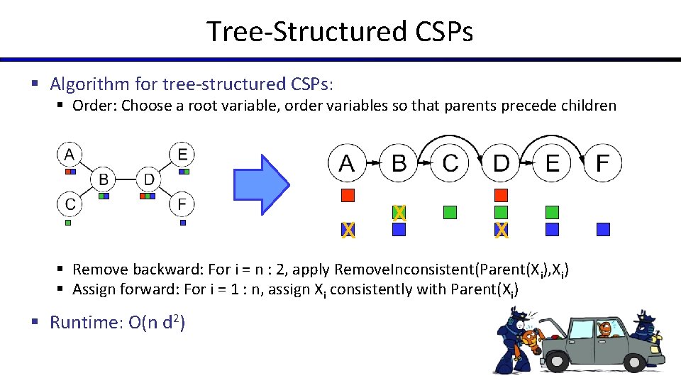
Tree-Structured CSPs § Algorithm for tree-structured CSPs: § Order: Choose a root variable, order variables so that parents precede children X X X § Remove backward: For i = n : 2, apply Remove. Inconsistent(Parent(Xi), Xi) § Assign forward: For i = 1 : n, assign Xi consistently with Parent(Xi) § Runtime: O(n d 2)

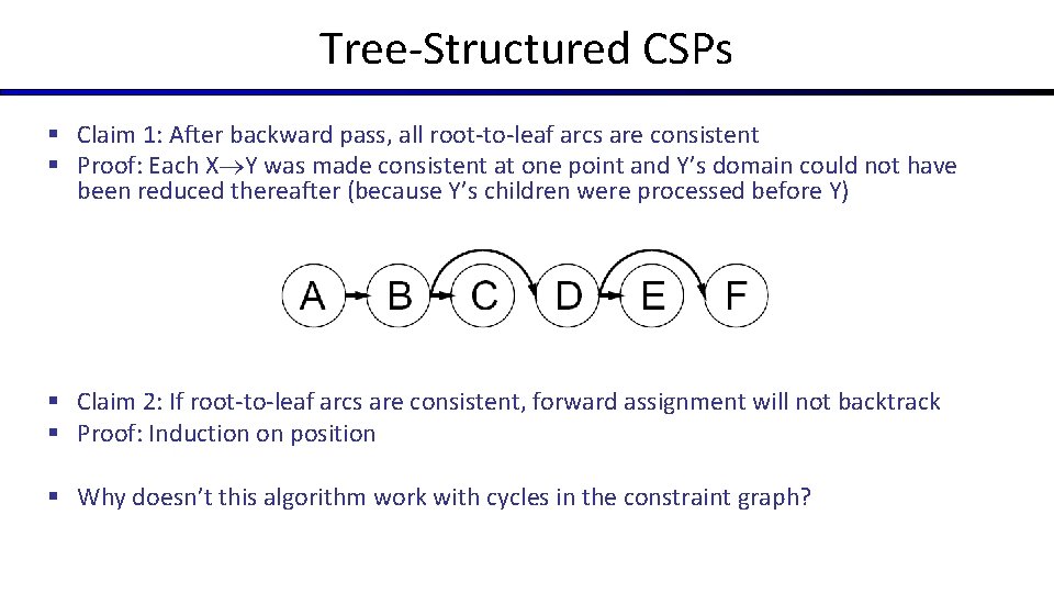
Tree-Structured CSPs § Claim 1: After backward pass, all root-to-leaf arcs are consistent § Proof: Each X Y was made consistent at one point and Y’s domain could not have been reduced thereafter (because Y’s children were processed before Y) § Claim 2: If root-to-leaf arcs are consistent, forward assignment will not backtrack § Proof: Induction on position § Why doesn’t this algorithm work with cycles in the constraint graph?

Improving Structure

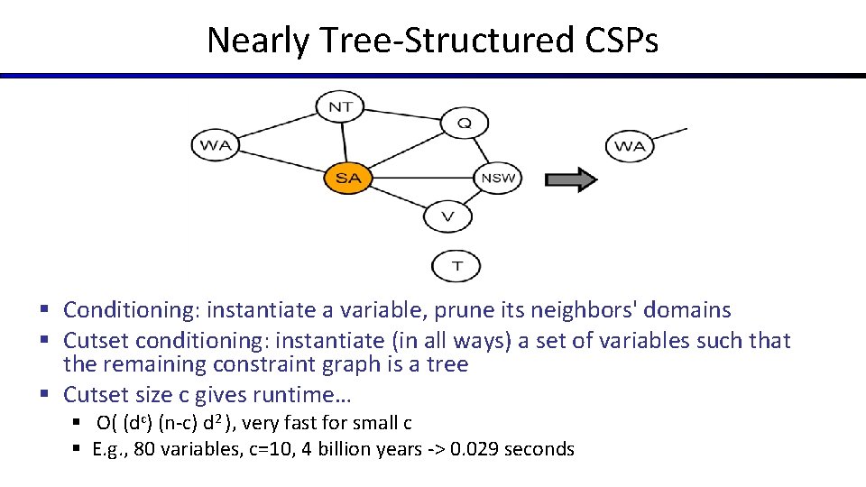
Nearly Tree-Structured CSPs § Conditioning: instantiate a variable, prune its neighbors' domains § Cutset conditioning: instantiate (in all ways) a set of variables such that the remaining constraint graph is a tree § Cutset size c gives runtime… § O( (dc) (n-c) d 2 ), very fast for small c § E. g. , 80 variables, c=10, 4 billion years -> 0. 029 seconds

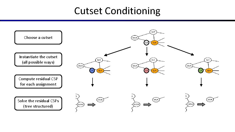
Cutset Conditioning Choose a cutset SA Instantiate the cutset (all possible ways) SA Compute residual CSP for each assignment Solve the residual CSPs (tree structured) SA SA

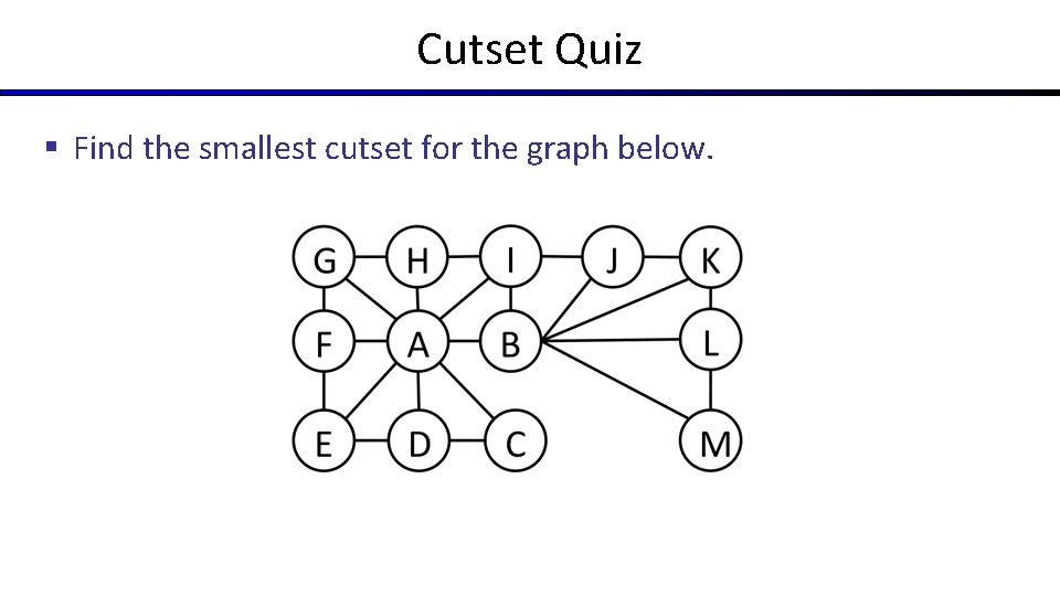
Cutset Quiz § Find the smallest cutset for the graph below.

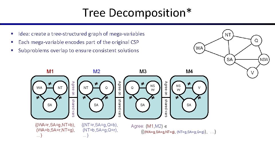
Tree Decomposition* § Idea: create a tree-structured graph of mega-variables § Each mega-variable encodes part of the original CSP § Subproblems overlap to ensure consistent solutions M 1 Q SA {(NT=r, SA=g, Q=b), (NT=b, SA=g, Q=r), …} Q NS W SA shared vars {(WA=r, SA=g, NT=b), (WA=b, SA=r, NT=g), …} M 4 Agree on SA NT shared vars NT M 3 Agree on WA M 2 NS W V SA Agree: (M 1, M 2) {((WA=g, SA=g, NT=g), (NT=g, SA=g, Q=g)), …}

Iterative Improvement

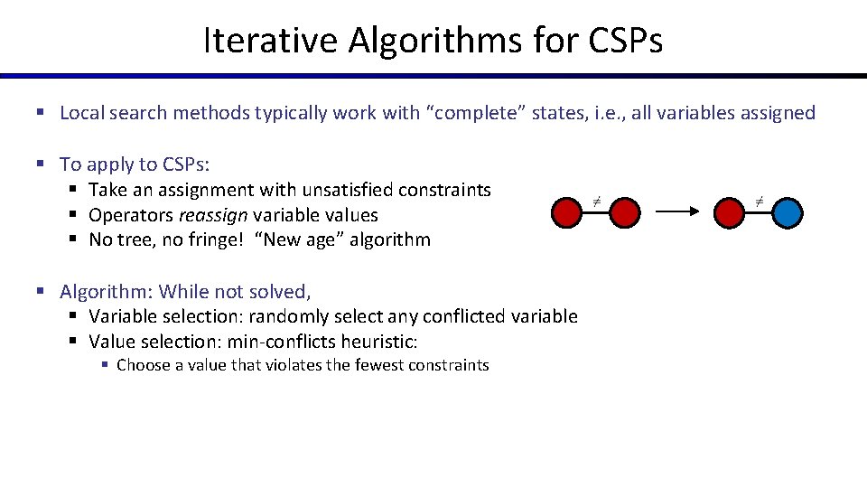
Iterative Algorithms for CSPs § Local search methods typically work with “complete” states, i. e. , all variables assigned § To apply to CSPs: § Take an assignment with unsatisfied constraints § Operators reassign variable values § No tree, no fringe! “New age” algorithm § Algorithm: While not solved, § Variable selection: randomly select any conflicted variable § Value selection: min-conflicts heuristic: § Choose a value that violates the fewest constraints

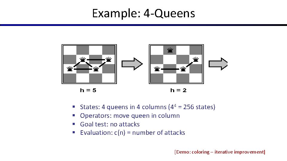
Example: 4 -Queens § § States: 4 queens in 4 columns (44 = 256 states) Operators: move queen in column Goal test: no attacks Evaluation: c(n) = number of attacks [Demo: coloring – iterative improvement]

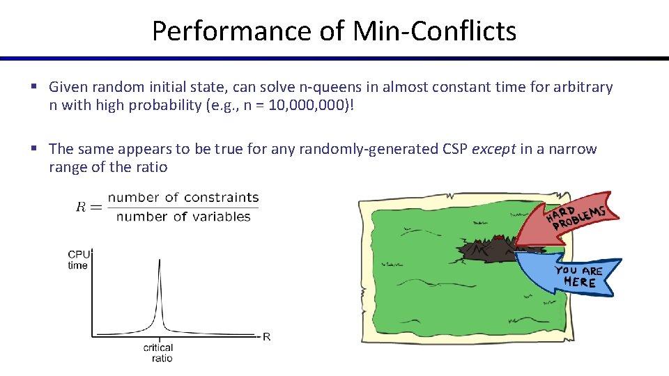
Performance of Min-Conflicts § Given random initial state, can solve n-queens in almost constant time for arbitrary n with high probability (e. g. , n = 10, 000)! § The same appears to be true for any randomly-generated CSP except in a narrow range of the ratio

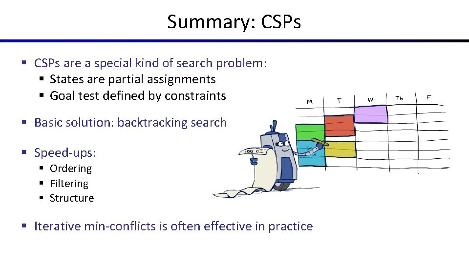
Summary: CSPs § CSPs are a special kind of search problem: § States are partial assignments § Goal test defined by constraints § Basic solution: backtracking search § Speed-ups: § Ordering § Filtering § Structure § Iterative min-conflicts is often effective in practice

Break quiz Given a search problem P expressed in the usual way: § initial state s 0, states S, actions A, goal test G, transition model Result(s, a) and a time horizon T, construct a CSP C such that C has a solution exactly when P has a solution of length T, and the solution to P can be read off from the solution to C Hint: You’ll need some variables for each time step, including At (the action taken at time t). What are the constraints between time steps? Other constraints on particular time steps?

Break quiz answer Variables of the CSP are § Action variables A 0 , …, AT-1 each with domain A § State variables S 0 , …, ST , each with domain S Constraints of the CSP are § S 0=s 0 § ST satisfies goal test G § For t=0, …, T-1, St+1=Result(St, At)

Local Search

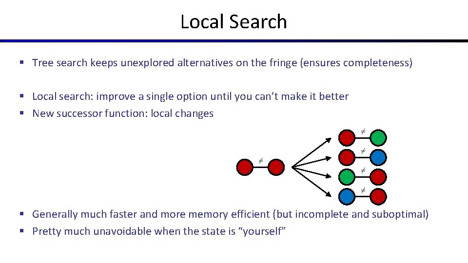
Local Search § Tree search keeps unexplored alternatives on the fringe (ensures completeness) § Local search: improve a single option until you can’t make it better § New successor function: local changes § Generally much faster and more memory efficient (but incomplete and suboptimal) § Pretty much unavoidable when the state is “yourself”

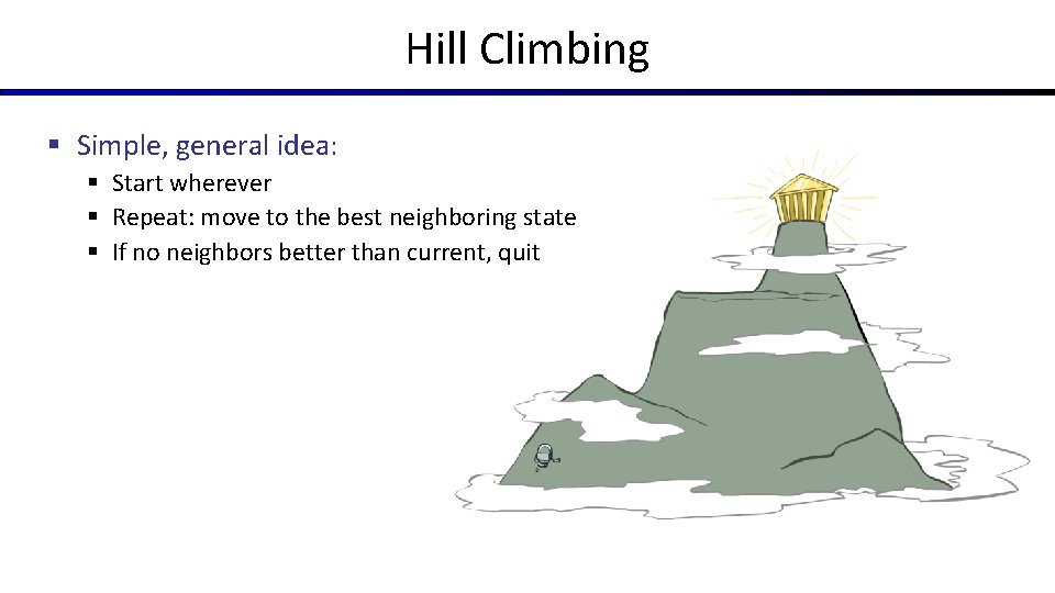
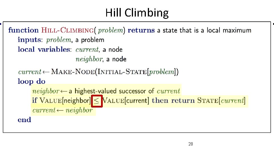
Hill Climbing § Simple, general idea: § Start wherever § Repeat: move to the best neighboring state § If no neighbors better than current, quit

Hill Climbing 28

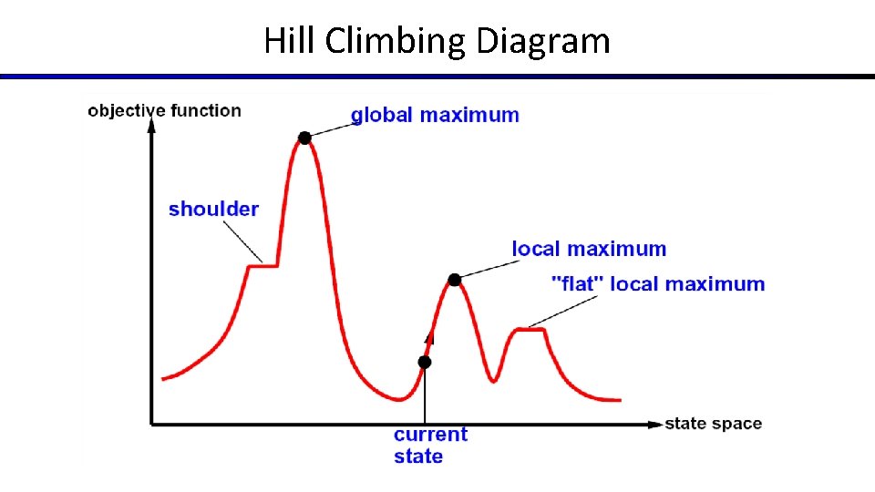
Hill Climbing Diagram

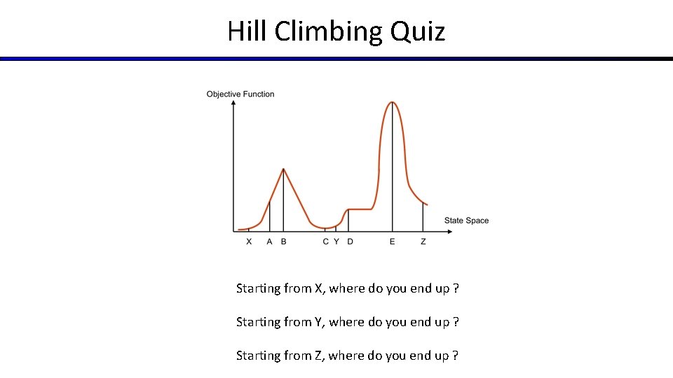
Hill Climbing Quiz Starting from X, where do you end up ? Starting from Y, where do you end up ? Starting from Z, where do you end up ?

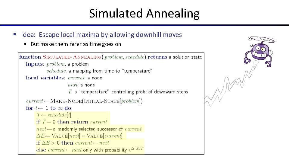
Simulated Annealing § Idea: Escape local maxima by allowing downhill moves § But make them rarer as time goes on 31

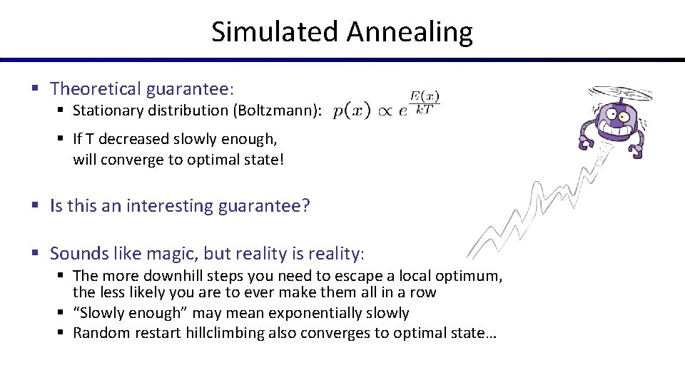
Simulated Annealing § Theoretical guarantee: § Stationary distribution (Boltzmann): § If T decreased slowly enough, will converge to optimal state! § Is this an interesting guarantee? § Sounds like magic, but reality is reality: § The more downhill steps you need to escape a local optimum, the less likely you are to ever make them all in a row § “Slowly enough” may mean exponentially slowly § Random restart hillclimbing also converges to optimal state…

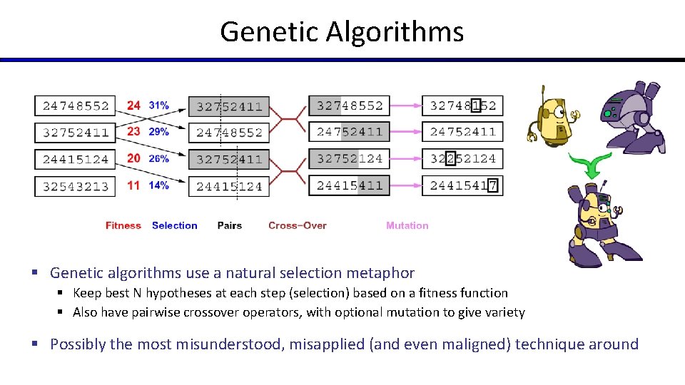
Genetic Algorithms § Genetic algorithms use a natural selection metaphor § Keep best N hypotheses at each step (selection) based on a fitness function § Also have pairwise crossover operators, with optional mutation to give variety § Possibly the most misunderstood, misapplied (and even maligned) technique around

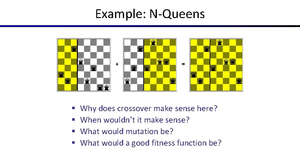
Example: N-Queens § § Why does crossover make sense here? When wouldn’t it make sense? What would mutation be? What would a good fitness function be?

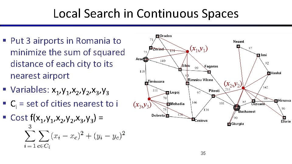
Local Search in Continuous Spaces § Put 3 airports in Romania to minimize the sum of squared distance of each city to its nearest airport § Variables: x 1, y 1, x 2, y 2, x 3, y 3 § Ci = set of cities nearest to i § Cost f(x 1, y 1, x 2, y 2, x 3, y 3) = (x 1, y 1) (x 2, y 2) (x 3, y 3) 35

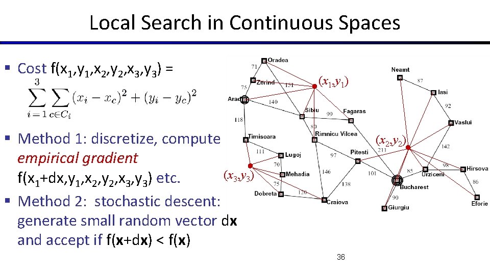
Local Search in Continuous Spaces § Cost f(x 1, y 1, x 2, y 2, x 3, y 3) = (x 1, y 1) § Method 1: discretize, compute empirical gradient (x 3, y 3) f(x 1+dx, y 1, x 2, y 2, x 3, y 3) etc. § Method 2: stochastic descent: generate small random vector dx and accept if f(x+dx) < f(x) (x 2, y 2) 36

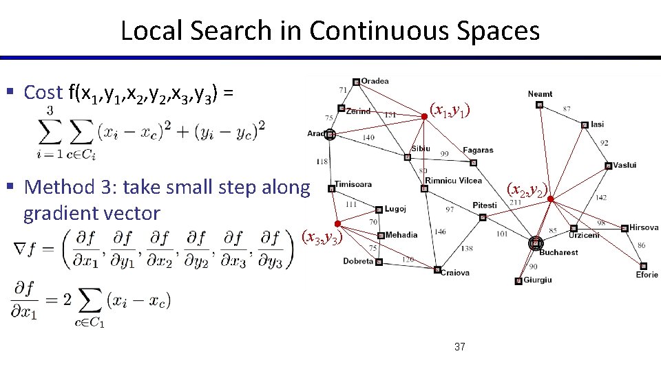
Local Search in Continuous Spaces § Cost f(x 1, y 1, x 2, y 2, x 3, y 3) = (x 1, y 1) § Method 3: take small step along gradient vector (x 2, y 2) (x 3, y 3) 37