Solvers for Mixed Integer Programming 600 325425 Declarative

Solvers for Mixed Integer Programming 600. 325/425 Declarative Methods - J. Eisner 1

Relaxation: A general optimization technique Want: n q q n x* = argminx f(x) subject to x S S is the feasible set Start by getting: q q x 1 = argminx f(x) subject to x T where S T n n q T is a larger feasible set, obtained by dropping some constraints Makes problem easier if we have a large # of constraints or difficult ones If we’re lucky, it happens that x 1 S n Then x* = x 1 , since q q q x 1 is a feasible solution to the original problem no feasible solution better than x 1 (no better x S since none anywhere T) Else, add some constraints back (to shrink T) and try again, getting x 2 n x 1, x 2, x 3, … x* as T closes in on S 600. 325/425 Declarative Methods - J. Eisner 2

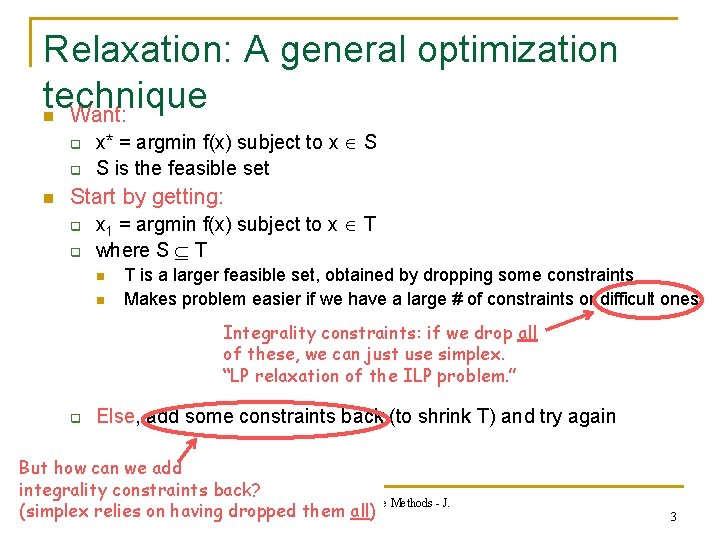
Relaxation: A general optimization technique Want: n q q n x* = argmin f(x) subject to x S S is the feasible set Start by getting: q q x 1 = argmin f(x) subject to x T where S T n n T is a larger feasible set, obtained by dropping some constraints Makes problem easier if we have a large # of constraints or difficult ones Integrality constraints: if we drop all of these, we can just use simplex. “LP relaxation of the ILP problem. ” q Else, add some constraints back (to shrink T) and try again But how can we add integrality constraints back? 600. 325/425 Declarative Methods - J. (simplex relies on having dropped them. Eisner all) 3

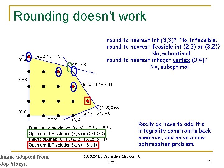
Rounding doesn’t work round to nearest int (3, 3)? No, infeasible. round to nearest feasible int (2, 3) or (3, 2)? No, suboptimal. round to nearest integer vertex (0, 4)? No, suboptimal. Really do have to add the integrality constraints back somehow, and solve a new optimization problem. image adapted from Jop Sibeyn 600. 325/425 Declarative Methods - J. Eisner 4

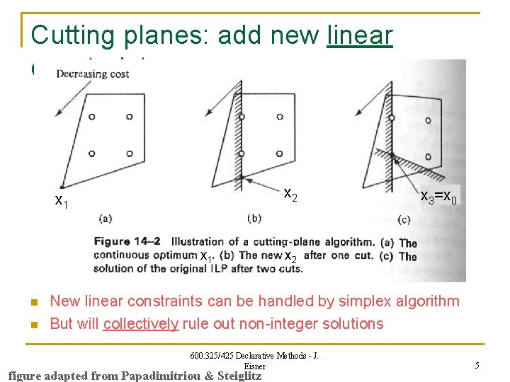
Cutting planes: add new linear constraints x 2 x 1 n n x 3=x 0 x 2 New linear constraints can be handled by simplex algorithm But will collectively rule out non-integer solutions 600. 325/425 Declarative Methods - J. Eisner figure adapted from Papadimitriou & Steiglitz 5

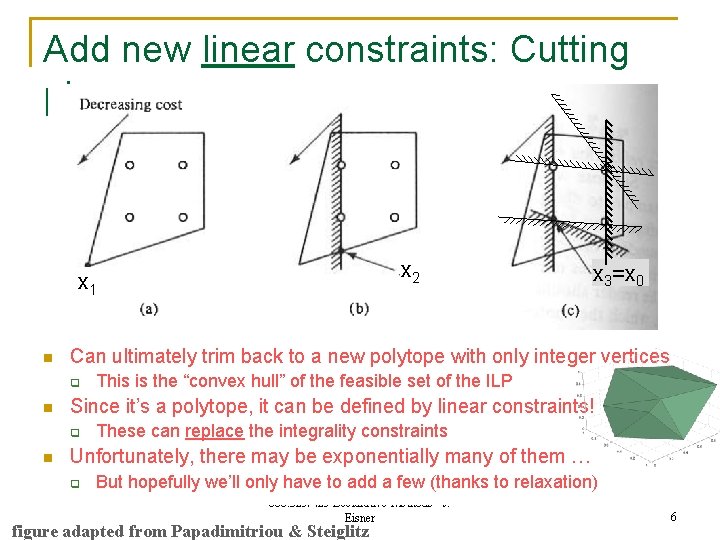
Add new linear constraints: Cutting planes x 2 x 1 n Can ultimately trim back to a new polytope with only integer vertices q n This is the “convex hull” of the feasible set of the ILP Since it’s a polytope, it can be defined by linear constraints! q n x 3=x 0 These can replace the integrality constraints Unfortunately, there may be exponentially many of them … q But hopefully we’ll only have to add a few (thanks to relaxation) 600. 325/425 Declarative Methods - J. Eisner figure adapted from Papadimitriou & Steiglitz 6

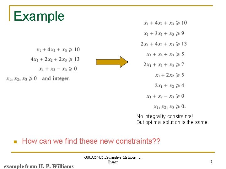
Example No integrality constraints! But optimal solution is the same. n How can we find these new constraints? ? example from H. P. Williams 600. 325/425 Declarative Methods - J. Eisner 7

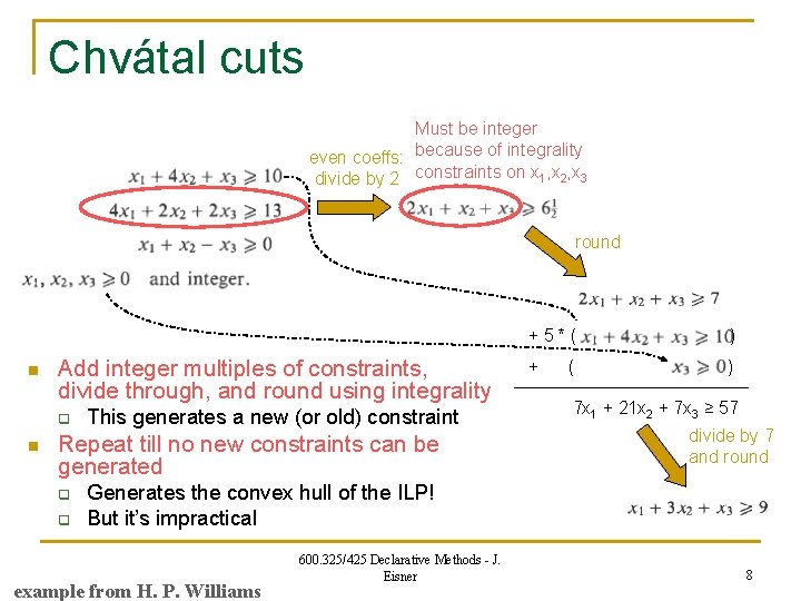
Chvátal cuts Must be integer even coeffs: because of integrality divide by 2 constraints on x 1, x 2, x 3 round n Add integer multiples of constraints, divide through, and round using integrality q n This generates a new (or old) constraint Repeat till no new constraints can be generated q q +5*( ) + ) ( 7 x 1 + 21 x 2 + 7 x 3 ≥ 57 divide by 7 and round Generates the convex hull of the ILP! But it’s impractical example from H. P. Williams 600. 325/425 Declarative Methods - J. Eisner 8

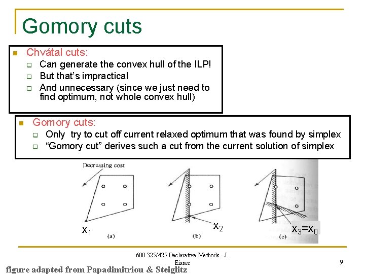
Gomory cuts Chvátal cuts: n Can generate the convex hull of the ILP! But that’s impractical And unnecessary (since we just need to find optimum, not whole convex hull) q q q n Gomory cuts: q q Only try to cut off current relaxed optimum that was found by simplex “Gomory cut” derives such a cut from the current solution of simplex x 2 x 1 600. 325/425 Declarative Methods - J. Eisner figure adapted from Papadimitriou & Steiglitz x 3=x 0 9

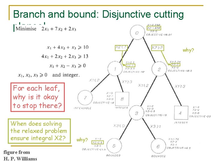
Branch and bound: Disjunctive cutting planes! why? For each leaf, why is it okay to stop there? When does solving the relaxed problem ensure integral X 2? figure from H. P. Williams why? 600. 325/425 Declarative Methods - J. Eisner 10

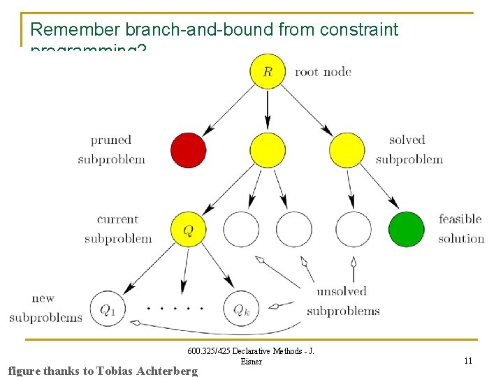
Remember branch-and-bound from constraint programming? 600. 325/425 Declarative Methods - J. Eisner figure thanks to Tobias Achterberg 11

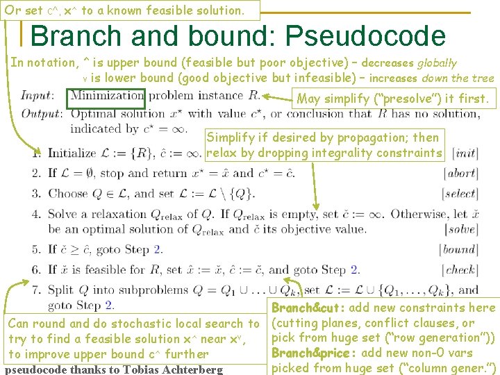
Or set c^, x^ to a known feasible solution. Branch and bound: Pseudocode In notation, ^ is upper bound (feasible but poor objective) – decreases globally v is lower bound (good objective but infeasible) – increases down the tree May simplify (“presolve”) it first. Simplify if desired by propagation; then relax by dropping integrality constraints Branch&cut: add new constraints here Can round and do stochastic local search to (cutting planes, conflict clauses, or pick from huge set (“row generation”)) try to find a feasible solution x^ near xv, 600. 325/425 Declarative Methods - J. Branch&price: add new non-0 vars to improve upper bound c^ further 12 Eisner picked from huge set (“column gener. ”) pseudocode thanks to Tobias Achterberg

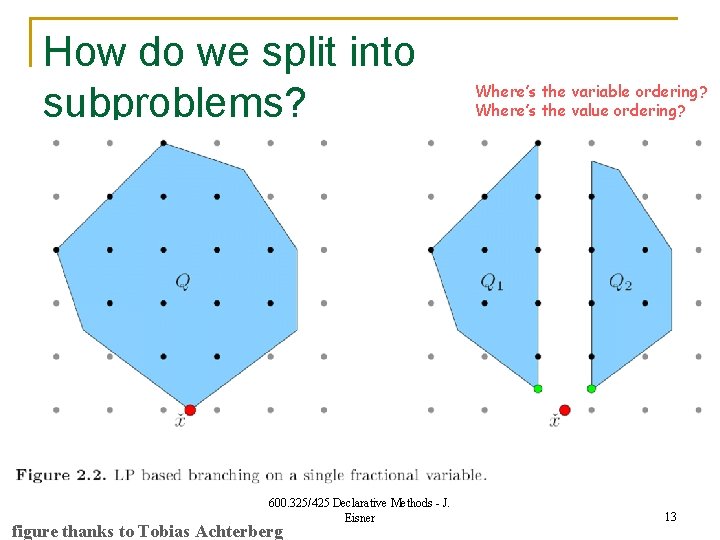
How do we split into subproblems? 600. 325/425 Declarative Methods - J. Eisner figure thanks to Tobias Achterberg Where’s the variable ordering? Where’s the value ordering? 13

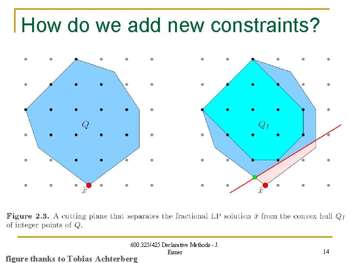
How do we add new constraints? 600. 325/425 Declarative Methods - J. Eisner figure thanks to Tobias Achterberg 14

Variable & value ordering heuristics (at a given node) n Priorities: User-specified var ordering n Most fractional branching: Branch on variable farthest from int n Branch on a variable that should tighten (hurt) the LP relaxation a lot q q q n Strong branching: For several candidate variables, try rounding them and solving the LP relaxation (perhaps incompletely). Penalties: If we rounded x up or down, how much would it tighten objective just on next iteration of dual simplex algorithm? (Dual simplex maintains an overly optimistic cost estimate that relaxes integrality and may be infeasible in other ways, too. ) Pseudo-costs: When rounding this variable in the past, how much has it actually tightened the LP relaxation objective (on average), per unit increase or decrease? Branching on SOS 1 and SOS 2 600. 325/425 Declarative Methods - J. Eisner 15

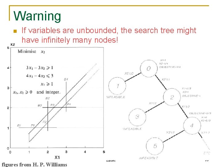
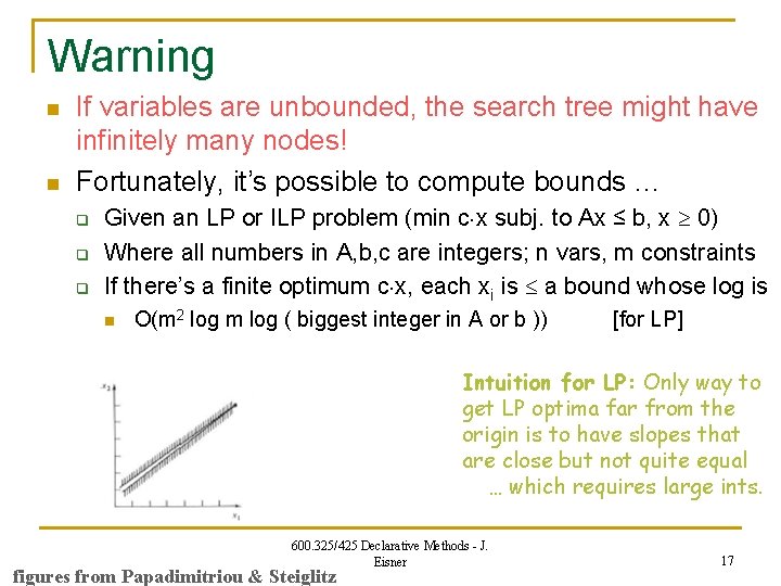
Warning n If variables are unbounded, the search tree might have infinitely many nodes! figures from H. P. Williams 600. 325/425 Declarative Methods - J. Eisner 16

Warning n n If variables are unbounded, the search tree might have infinitely many nodes! Fortunately, it’s possible to compute bounds … q q q Given an LP or ILP problem (min c x subj. to Ax ≤ b, x 0) Where all numbers in A, b, c are integers; n vars, m constraints If there’s a finite optimum c x, each xi is a bound whose log is n O(m 2 log m log ( biggest integer in A or b )) [for LP] Intuition for LP: Only way to get LP optima far from the origin is to have slopes that are close but not quite equal … which requires large ints. 600. 325/425 Declarative Methods - J. Eisner figures from Papadimitriou & Steiglitz 17

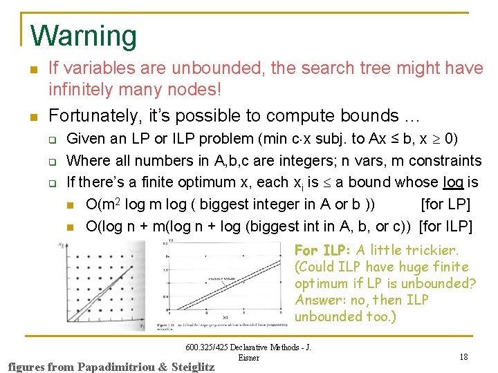
Warning n n If variables are unbounded, the search tree might have infinitely many nodes! Fortunately, it’s possible to compute bounds … q q q Given an LP or ILP problem (min c x subj. to Ax ≤ b, x 0) Where all numbers in A, b, c are integers; n vars, m constraints If there’s a finite optimum x, each xi is a bound whose log is n O(m 2 log m log ( biggest integer in A or b )) [for LP] n O(log n + m(log n + log (biggest in A, b, or c)) [for ILP] For ILP: A little trickier. (Could ILP have huge finite optimum if LP is unbounded? Answer: no, then ILP unbounded too. ) 600. 325/425 Declarative Methods - J. Eisner figures from Papadimitriou & Steiglitz 18

Reducing ILP to 0 -1 ILP q q q Given an LP or ILP problem (min c. x subj. to Ax=b, x 0) Where all numbers in A, b, c are integers; n vars, m constraints If there’s a finite optimum x, each xi is a bound whose log is n n n If log bound=100, then e. g. 0 x 5 2100 Remark: This bound enables a polytime reduction from ILP to 0 -1 ILP q n n n O(log n + m(log n + log (biggest in A, b, or c)) [for ILP] Remember: Size of problem = length of encoding, not size of #s Can you see how? Hint: Binary numbers are encoded with 0 and 1 What happens to linear function like …+ 3 x 5 + … ? 600. 325/425 Declarative Methods - J. Eisner 19

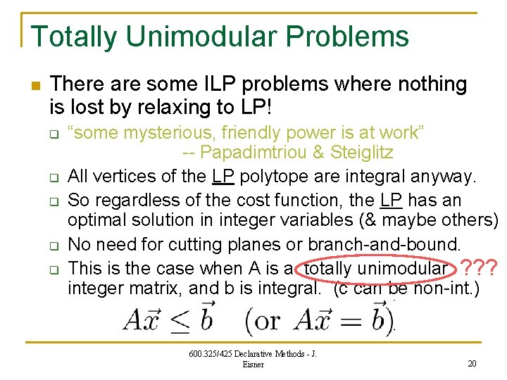
Totally Unimodular Problems n There are some ILP problems where nothing is lost by relaxing to LP! q q q “some mysterious, friendly power is at work” -- Papadimtriou & Steiglitz All vertices of the LP polytope are integral anyway. So regardless of the cost function, the LP has an optimal solution in integer variables (& maybe others) No need for cutting planes or branch-and-bound. This is the case when A is a totally unimodular ? ? ? integer matrix, and b is integral. (c can be non-int. ) 600. 325/425 Declarative Methods - J. Eisner 20

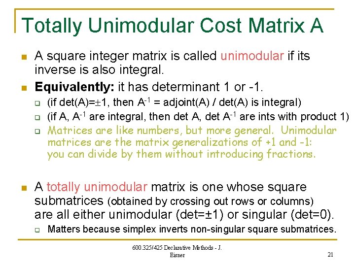
Totally Unimodular Cost Matrix A n n A square integer matrix is called unimodular if its inverse is also integral. Equivalently: it has determinant 1 or -1. q q q n (if det(A)= 1, then A-1 = adjoint(A) / det(A) is integral) (if A, A-1 are integral, then det A, det A-1 are ints with product 1) Matrices are like numbers, but more general. Unimodular matrices are the matrix generalizations of +1 and -1: you can divide by them without introducing fractions. A totally unimodular matrix is one whose square submatrices (obtained by crossing out rows or columns) are all either unimodular (det=± 1) or singular (det=0). q Matters because simplex inverts non-singular square submatrices. 600. 325/425 Declarative Methods - J. Eisner 21

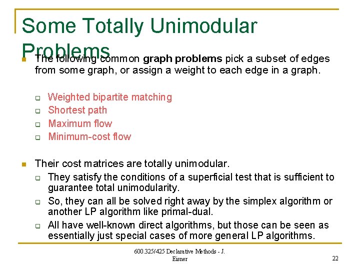
Some Totally Unimodular Problems The following common graph problems pick a subset of edges n from some graph, or assign a weight to each edge in a graph. q q n Weighted bipartite matching Shortest path Maximum flow Minimum-cost flow Their cost matrices are totally unimodular. q They satisfy the conditions of a superficial test that is sufficient to guarantee total unimodularity. q So, they can all be solved right away by the simplex algorithm or another LP algorithm like primal-dual. q All have well-known direct algorithms, but those can be seen as essentially just special cases of more general LP algorithms. 600. 325/425 Declarative Methods - J. Eisner 22

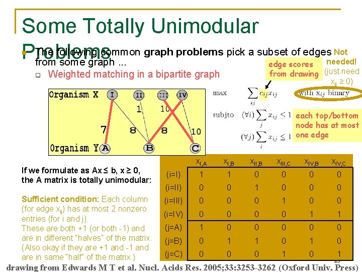
Some Totally Unimodular The following common graph problems pick a subset of edges Problems from some graph. . . Not needed! edge scores from drawing (just need xij ≥ 0) n q Weighted matching in a bipartite graph each top/bottom node has at most one edge x. I, A x. I, B x. III, C x. IV, B x. IV, C (i=I) 1 1 0 0 (i=II) 0 0 1 0 0 0 Sufficient condition: Each column (i=III) 0 0 (for edge xij) has at most 2 nonzero (i=IV) 0 0 entries (for i and j). (j=A) 1 0 These are both +1 (or both -1) and are in different “halves” of the matrix. (j=B) 0 1 (Also okay if they are +1 and -1 and 600. 325/425(j=C) Declarative Methods - J. 0 0 are in same “half” of the matrix. ) Eisner 0 1 0 0 0 0 1 0 1 0 If we formulate as Ax ≤ b, x ≥ 0, the A matrix is totally unimodular: 1 23 drawing from Edwards M T et al. Nucl. Acids Res. 2005; 33: 3253 -3262 (Oxford Univ. Press)

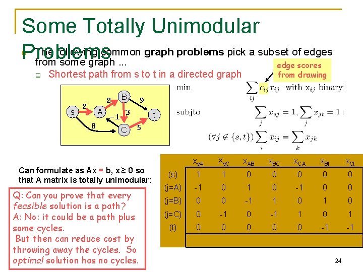
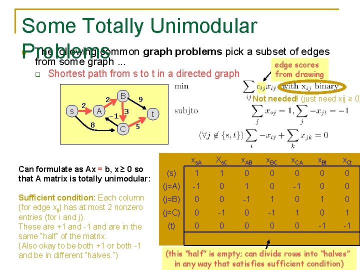
Some Totally Unimodular The following common graph problems pick a subset of edges Problems from some graph. . . n q edge scores from drawing Shortest path from s to t in a directed graph s 2 2 A 8 -1 B 9 3 C t 5 Can formulate as Ax = b, x ≥ 0 so that A matrix is totally unimodular: xs. A Xs. C x. AB x. BC x. CA x. Bt x. Ct (s) 1 1 0 0 0 (j=A) -1 0 0 -1 1 0 1 0 0 0 -1 -1 Q: Can you prove that every (j=B) 0 0 feasible solution is a path? (j=C) 0 -1 A: No: it could be a path plus (t) 0 0 some cycles. But then can reduce cost by throwing away the cycles. So 600. 325/425 Declarative Methods - J. Eisner optimal solution has no cycles. 24

Some Totally Unimodular The following common graph problems pick a subset of edges Problems from some graph. . . n q edge scores from drawing Shortest path from s to t in a directed graph s 2 2 A 8 -1 B 3 C Not needed! (just need xij ≥ 0) 9 t 5 Can formulate as Ax = b, x ≥ 0 so that A matrix is totally unimodular: xs. A Xs. C x. AB x. BC x. CA x. Bt x. Ct (s) 1 1 0 0 0 (j=A) -1 0 0 Sufficient condition: Each column (j=B) 0 0 -1 1 0 (for edge xij) has at most 2 nonzero (j=C) 0 -1 1 0 1 entries (for i and j). (t) 0 0 0 -1 -1 These are +1 and -1 and are in the same “half” of the matrix. (Also okay to be both +1 or both -1 600. 325/425 Declarative Methods - J. (this “half” is empty; can divide rows into “halves” and be in different “halves. ”) Eisner 25 in any way that satisfies sufficient condition)

Some Totally Unimodular The following common graph problems pick a subset of edges from Problems some graph. . . n q q n n Maximum flow (previous problems can be reduced to this) Minimum-cost flow Cost matrix is rather similar to those on the previous slides, but with additional “capacity constraints” like xij ≤ kij Fortunately, if A is totally unimodular, so is A with I (the identity matrix) glued underneath it to represent the additional constraints

Solving Linear Programs 600. 325/425 Declarative Methods - J. Eisner 27

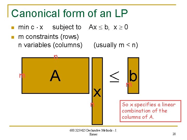
Canonical form of an LP n n min c x subject to Ax b, x 0 m constraints (rows) n variables (columns) (usually m < n) n m A x mb n 600. 325/425 Declarative Methods - J. Eisner So x specifies a linear combination of the columns of A. 28

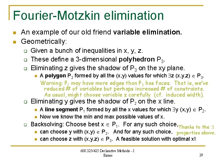
Fourier-Motzkin elimination n n An example of our old friend variable elimination. Geometrically: q q q Given a bunch of inequalities in x, y, z. These define a 3 -dimensional polyhedron P 3. Eliminating z gives the shadow of P 3 on the xy plane. n q Eliminating y gives the shadow of P 2 on the x line. n n q A polygon P 2 formed by all the (x, y) values for which z (x, y, z) P 3. Warning: P 2 may have more edges than P 3 has faces. That is, we’ve reduced # of variables but perhaps increased # of constraints. As usual, might choose variable z carefully (cf. induced width). A line segment P 1 formed by all the x values for which y (x, y) P 2. Now we know the min and max possible values of x. Backsolving: Choose best x P 1. For any such choice, Thanks to the n n can choose y with (x, y) P 2. And for any such choice, properties above. can choose z with (x, y, z) P 3. A feasible solution with optimal x! 600. 325/425 Declarative Methods - J. Eisner 29

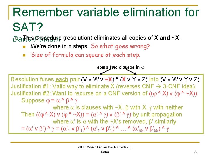
Remember variable elimination for SAT? q This procedure (resolution) eliminates all copies of X and ~X. Davis-Putnam n n We’re done in n steps. So what goes wrong? Size of formula can square at each step. some two clauses in Resolution fuses each pair (V v W v ~X) ^ (X v Y v Z) into (V v W v Y v Z) Justification #1: Valid way to eliminate X (reverses CNF 3 -CNF idea). Justification #2: Want to recurse on a CNF version of (( ^ X) v ( ^ ~X)) Suppose = ^ ^ where is clauses with ~X, with neither Then (( ^ X) v ( ^ ~X)) = ( ’ ^ ) v ( ’ ^ ) by unit propagation where ’ is with the ~X’s removed, ’ similarly. = ( ’ v ’) ^ = ( ’ 1 v ’ 1) ^ ( ’ 1 v ’ 2) ^ … ^ ( ’ 99 v ’ 99) ^ 600. 325/425 Declarative Methods - J. Eisner 30

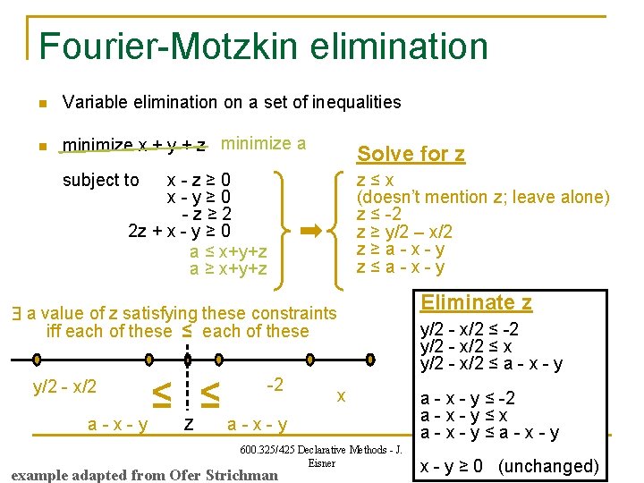
Fourier-Motzkin elimination n Variable elimination on a set of inequalities n minimize x + y + z minimize a Solve for z subject to z≤x (doesn’t mention z; leave alone) z ≤ -2 z ≥ y/2 – x/2 z≥a-x-y z≤a-x-y x-z≥ 0 x-y≥ 0 -z≥ 2 2 z + x - y ≥ 0 a ≤ x+y+z a ≥ x+y+z a value of z satisfying these constraints iff each of these ≤ each of these y/2 - x/2 a-x-y ≤ ≤ z -2 x a-x-y 600. 325/425 Declarative Methods - J. Eisner example adapted from Ofer Strichman Eliminate z y/2 - x/2 ≤ -2 y/2 - x/2 ≤ x y/2 - x/2 ≤ a - x - y ≤ -2 a-x-y≤x a-x-y≤a-x-y x - y ≥ 0 (unchanged)31

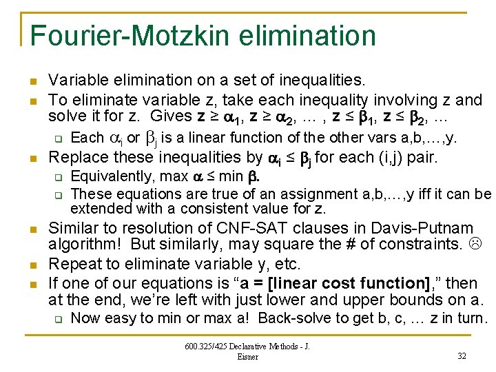
Fourier-Motzkin elimination n n Variable elimination on a set of inequalities. To eliminate variable z, take each inequality involving z and solve it for z. Gives z ≥ 1, z ≥ 2, … , z ≤ 1, z ≤ 2, … q n Replace these inequalities by i ≤ j for each (i, j) pair. q q n n n Each i or j is a linear function of the other vars a, b, …, y. Equivalently, max ≤ min . These equations are true of an assignment a, b, …, y iff it can be extended with a consistent value for z. Similar to resolution of CNF-SAT clauses in Davis-Putnam algorithm! But similarly, may square the # of constraints. Repeat to eliminate variable y, etc. If one of our equations is “a = [linear cost function], ” then at the end, we’re left with just lower and upper bounds on a. q Now easy to min or max a! Back-solve to get b, c, … z in turn. 600. 325/425 Declarative Methods - J. Eisner 32

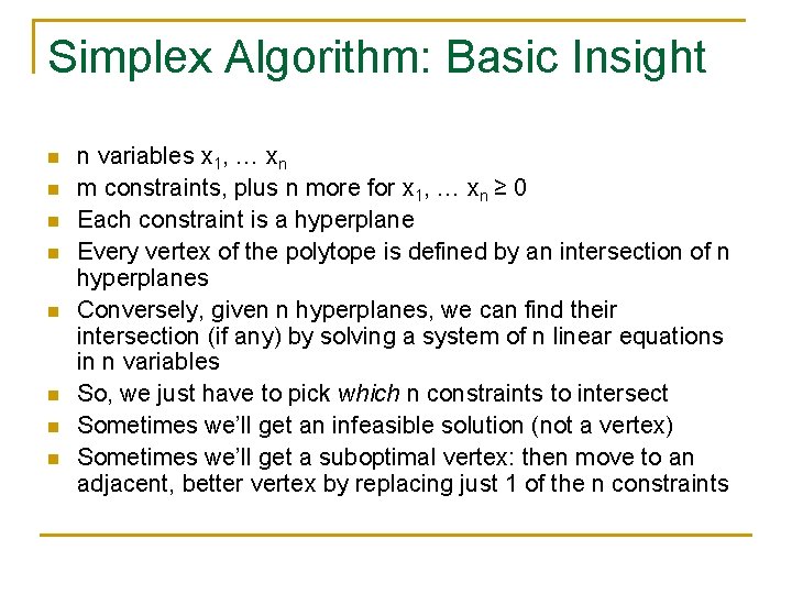
Simplex Algorithm: Basic Insight n n n n n variables x 1, … xn m constraints, plus n more for x 1, … xn ≥ 0 Each constraint is a hyperplane Every vertex of the polytope is defined by an intersection of n hyperplanes Conversely, given n hyperplanes, we can find their intersection (if any) by solving a system of n linear equations in n variables So, we just have to pick which n constraints to intersect Sometimes we’ll get an infeasible solution (not a vertex) Sometimes we’ll get a suboptimal vertex: then move to an adjacent, better vertex by replacing just 1 of the n constraints

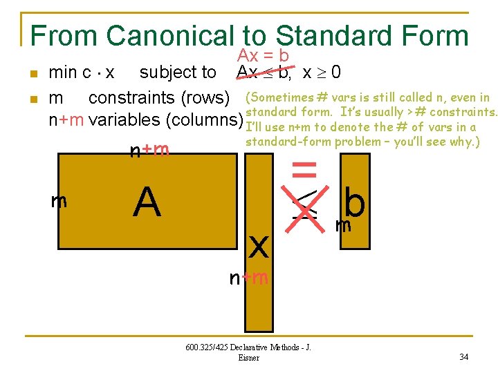
From Canonical to Standard Form n n Ax = b Ax b, x 0 min c x subject to m constraints (rows) (Sometimes # vars is still called n, even in standard form. It’s usually > # constraints. n+m variables (columns) I’ll use n+m to denote the # of vars in a n +m m A standard-form problem – you’ll see why. ) x = mb n+m 600. 325/425 Declarative Methods - J. Eisner 34

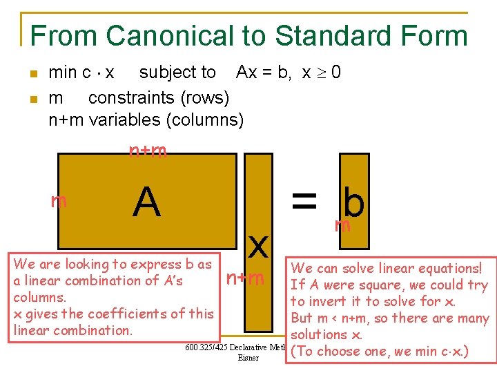
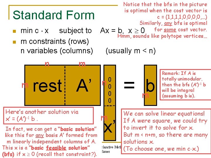
From Canonical to Standard Form n n min c x subject to Ax = b, x 0 m constraints (rows) n+m variables (columns) n+m m A We are looking to express b as a linear combination of A’s columns. x gives the coefficients of this linear combination. x = mb We can solve linear equations! If A were square, we could try to invert it to solve for x. But m < n+m, so there are many solutions x. 600. 325/425 Declarative Methods - J. (To choose one, we min c x. ) 35 Eisner n+m

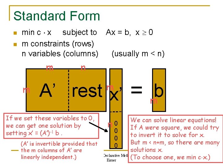
Standard Form n n min c x subject to Ax = b, x 0 m constraints (rows) n variables (columns) (usually m < n) m m n m A’ rest x’ If we set these variables to 0, we can get one solution by setting x’ = (A’)-1 b. = mb We can solve linear equations! If A were square, we could try to invert it to solve for x. But m < n+m, so there are many (A’ is invertible provided that solutions x. the m columns of A’ are Methods - J. linearly independent. ) 600. 325/425 Declarative (To choose one, we min c x. ) 36 Eisner n 0 0

Notice that the bfs in the picture is optimal when the cost vector is c = (1, 1, 0, 0, …) Similarly, any bfs is optimal b, x 0 for some cost vector. Hmm, sounds like polytope vertices… Standard Form n n min c x subject to Ax = m constraints (rows) n variables (columns) (usually m < n) n m m rest A’ Here’s another solution via x’ = (A’)-1 b. n 00 0 0 = mb Remark: If A is totally unimodular, then the bfs (A’)-1 b will be integral (assuming b is). We can solve linear equations! If A were square, we could try to invert it to solve for x. In fact, we can get a “basic solution” But m < n+m, so there are many like this for any basis A’ formed from m linearly independent columns of A. solutions x. 600. 325/425 Declarative Methods - J. This x is a “basic feasible solution” (To choose one, we min c x. ) 37 Eisner (bfs) if x 0 (recall that constraint? ). m x’

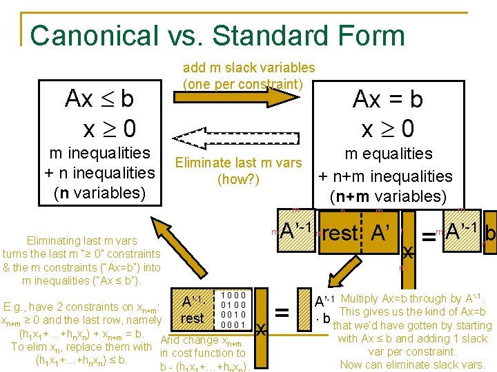
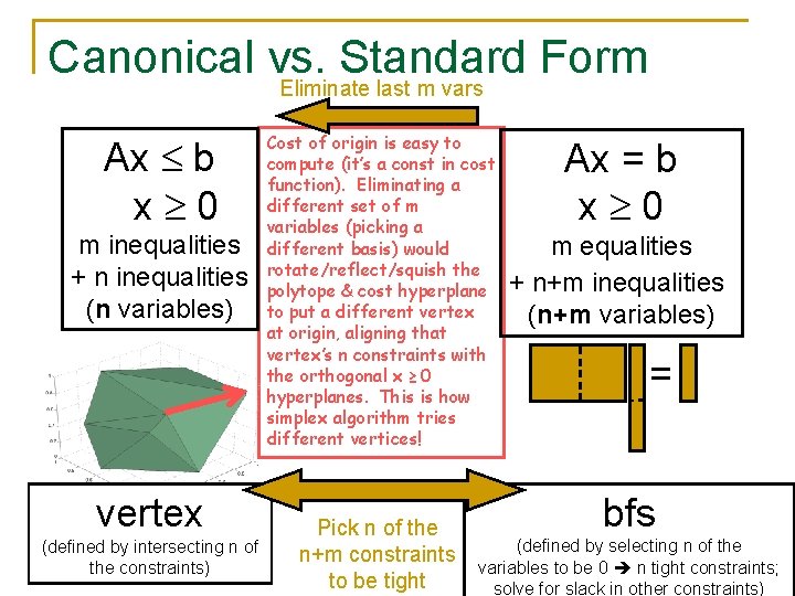
Canonical vs. Standard Form Ax b x 0 m inequalities + n inequalities (n variables) add m slack variables (one per constraint) Eliminate last m vars (how? ) m m Eliminating last m vars turns the last m “≥ 0” constraints & the m constraints (“Ax=b”) into m inequalities (“Ax ≤ b”). Ax = b x 0 m equalities + n+m inequalities (n+m variables) n m A’-1 mrest A’ = x n m m A’-1 mb m A’-1 rest 1000 0100 0010 0001 E. g. , have 2 constraints on xn+m: xn+m ≥ 0 and the last row, namely (h 1 x 1+…+hnxn) + xn+m = b. And change xn+m To elim xn, replace them with in cost function to (h 1 x 1+…+hnxn) ≤ b. b - (h x +…+h x ). = x A’-1 Multiply Ax=b through by A’. This gives us the kind of Ax=b b that we’d have gotten by starting -1 with Ax ≤ b and adding 1 slack var per constraint. Now can eliminate slack vars.

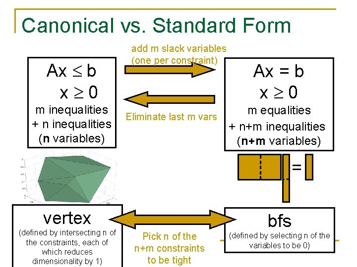
Canonical vs. Standard Form Ax b x 0 m inequalities + n inequalities (n variables) add m slack variables (one per constraint) Eliminate last m vars Ax = b x 0 m equalities + n+m inequalities (n+m variables) = vertex (defined by intersecting n of the constraints, each of which reduces dimensionality by 1) bfs Pick n of the n+m constraints to be tight (defined by selecting n of the variables to be 0)

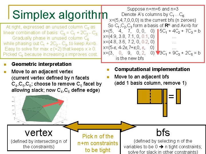
Suppose n+m=6 and n=3 Denote A’s columns by C 1…C 6 x=(5, 4, 7, 0, 0, 0) is the current bfs (n zeroes) So C 1, C 2, C 3 form a basis of Rm and Ax=b for x=(5, 4, 7, 0, 0, 0) 5 C 1 + 4 C 2 + 7 C 3 = b x=(4. 9, 3. 8, 7. 1, 0, 0. 1, 0) … x=(4. 8, 3. 6, 7. 2, 0, 0. 2, 0) … x=(5 - , 4 -2 , 7+ , 0, , 0) … x=(3, 0, 9, 0, 2, 0) 3 C 1 + 9 C 3 + 2 C 5 = b is the new bfs Simplex algorithm At right, expressed an unused column C 5 as linear combination of basis: C 5 = C 1 + 2 C 2 - C 3. Gradually phase in unused column C 5 while phasing out C 1 + 2 C 2 - C 3, to keep Ax=b. Easy to solve for max (=2) that keeps x ≥ 0. Picked C 5 because increasing improves cost. n n Geometric interpretation Move to an adjacent vertex (current vertex defined by n facets C 4, C 5, C 6; choose to remove C 5 facet by allowing slack; now C 4, C 6 define edge) vertex (defined by intersecting n of the constraints) n n Computational implementation Move to an adjacent bfs (add 1 basis column, remove 1) Pick n of the n+m constraints to be tight = bfs (defined by selecting n of the variables to be 0 n tight constraints; solve for slack in other constraints)

Canonical vs. Standard Form Eliminate last m vars Ax b x 0 m inequalities + n inequalities (n variables) vertex (defined by intersecting n of the constraints) Cost of origin is easy to compute (it’s a const in cost function). Eliminating a different set of m variables (picking a different basis) would rotate/reflect/squish the polytope & cost hyperplane to put a different vertex at origin, aligning that vertex’s n constraints with the orthogonal x ≥ 0 hyperplanes. This is how simplex algorithm tries different vertices! Pick n of the n+m constraints to be tight Ax = b x 0 m equalities + n+m inequalities (n+m variables) = bfs (defined by selecting n of the variables to be 0 n tight constraints; solve for slack in other constraints)

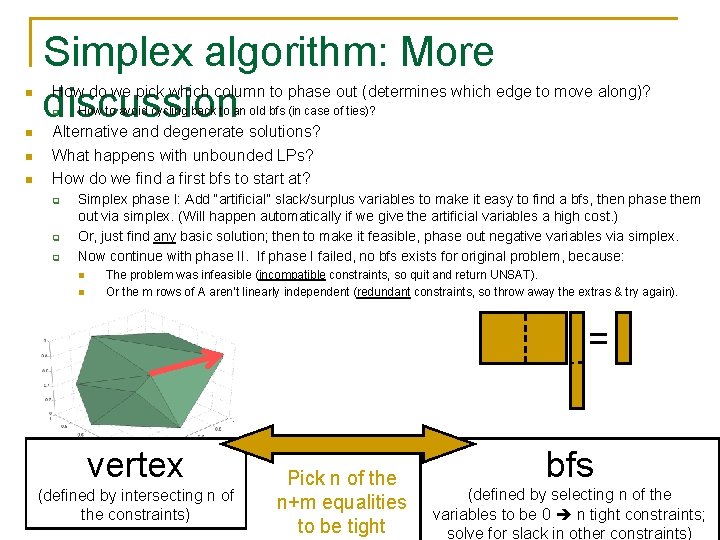
n Simplex algorithm: More discussion How do we pick which column to phase out (determines which edge to move along)? q n n n How to avoid cycling back to an old bfs (in case of ties)? Alternative and degenerate solutions? What happens with unbounded LPs? How do we find a first bfs to start at? q q q Simplex phase I: Add “artificial” slack/surplus variables to make it easy to find a bfs, then phase them out via simplex. (Will happen automatically if we give the artificial variables a high cost. ) Or, just find any basic solution; then to make it feasible, phase out negative variables via simplex. Now continue with phase II. If phase I failed, no bfs exists for original problem, because: n n The problem was infeasible (incompatible constraints, so quit and return UNSAT). Or the m rows of A aren’t linearly independent (redundant constraints, so throw away the extras & try again). = vertex (defined by intersecting n of the constraints) Pick n of the n+m equalities to be tight bfs (defined by selecting n of the variables to be 0 n tight constraints; solve for slack in other constraints)

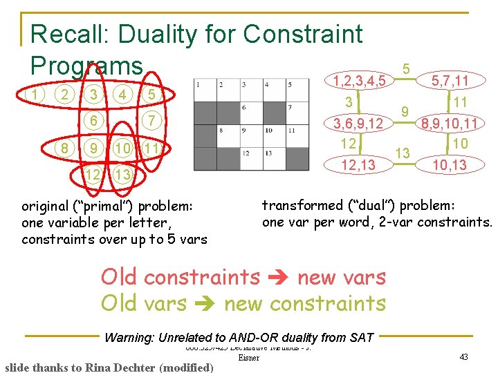
Recall: Duality for Constraint Programs 1, 2, 3, 4, 5 1 2 8 3 4 5 6 7 9 10 11 12 3 3, 6, 9, 12 12 12, 13 13 original (“primal”) problem: one variable per letter, constraints over up to 5 vars 5 9 13 5, 7, 11 11 8, 9, 10, 11 10 10, 13 transformed (“dual”) problem: one var per word, 2 -var constraints. Old constraints new vars Old vars new constraints Warning: Unrelated to AND-OR duality from SAT 600. 325/425 Declarative Methods - J. Eisner slide thanks to Rina Dechter (modified) 43

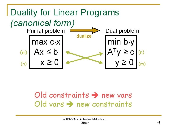
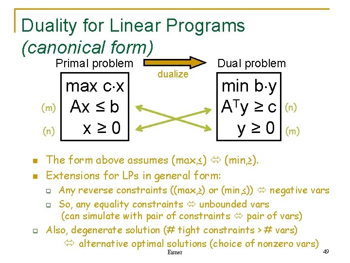
Duality for Linear Programs (canonical form) Primal problem (m) (n) max c x Ax ≤ b x≥ 0 dualize Dual problem min b y A Ty ≥ c y≥ 0 (n) (m) Old constraints new vars Old vars new constraints 600. 325/425 Declarative Methods - J. Eisner 44

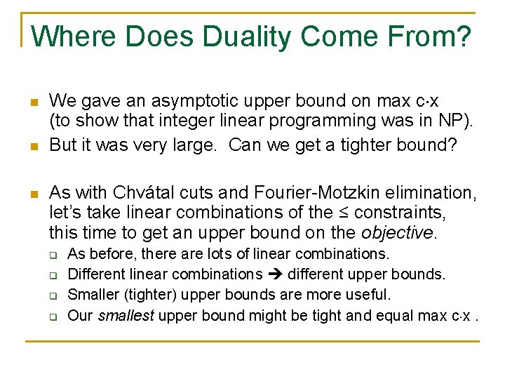
Where Does Duality Come From? n n n We gave an asymptotic upper bound on max c x (to show that integer linear programming was in NP). But it was very large. Can we get a tighter bound? As with Chvátal cuts and Fourier-Motzkin elimination, let’s take linear combinations of the ≤ constraints, this time to get an upper bound on the objective. q q As before, there are lots of linear combinations. Different linear combinations different upper bounds. Smaller (tighter) upper bounds are more useful. Our smallest upper bound might be tight and equal max c x.

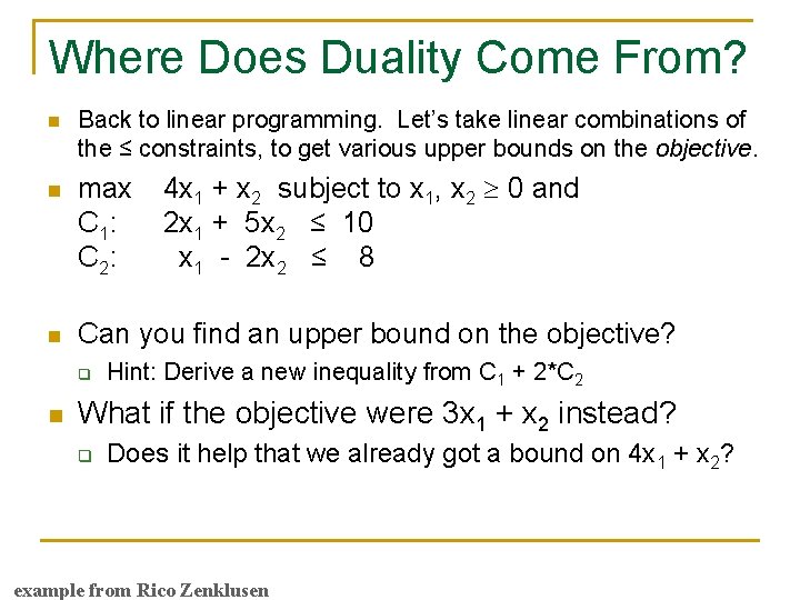
Where Does Duality Come From? n Back to linear programming. Let’s take linear combinations of the ≤ constraints, to get various upper bounds on the objective. 4 x 1 + x 2 subject to x 1, x 2 0 and 2 x 1 + 5 x 2 ≤ 10 x 1 - 2 x 2 ≤ 8 n max C 1: C 2: n Can you find an upper bound on the objective? q n Hint: Derive a new inequality from C 1 + 2*C 2 What if the objective were 3 x 1 + x 2 instead? q Does it help that we already got a bound on 4 x 1 + x 2? example from Rico Zenklusen

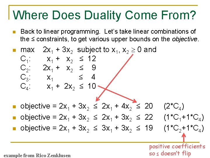
Where Does Duality Come From? n Back to linear programming. Let’s take linear combinations of the ≤ constraints, to get various upper bounds on the objective. 2 x 1 + 3 x 2 subject to x 1, x 2 0 and x 1 + x 2 ≤ 12 2 x 1 + x 2 ≤ 9 x 1 ≤ 4 x 1 + 2 x 2 ≤ 10 n max C 1: C 2: C 3: C 4: n objective = 2 x 1 + 3 x 2 ≤ 2 x 1 + 4 x 2 ≤ 20 objective = 2 x 1 + 3 x 2 ≤ 22 objective = 2 x 1 + 3 x 2 ≤ 3 x 1 + 3 x 2 ≤ 19 n n example from Rico Zenklusen (2*C 4) (1*C 1+1*C 4) (1*C 2+1*C 4) positive coefficients so ≤ doesn’t flip

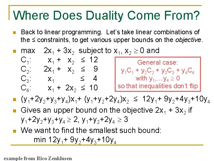
Where Does Duality Come From? n n n Back to linear programming. Let’s take linear combinations of the ≤ constraints, to get various upper bounds on the objective. max 2 x 1 + 3 x 2 subject to x 1, x 2 0 and C 1: x 1 + x 2 ≤ 12 General case: C 2: 2 x 1 + x 2 ≤ 9 y 1 C 1 + y 2 C 2 + y 3 C 3 + y 4 C 4 with y 1, …y 4 0 C 3: x 1 ≤ 4 so that inequalities don’t flip C 4: x 1 + 2 x 2 ≤ 10 (y 1+2 y 2+y 3+y 4)x 1+ (y 1+y 2+2 y 4)x 2 ≤ 12 y 1+ 9 y 2+4 y 3+10 y 4 Gives an upper bound on the objective 2 x 1 + 3 x 2 if y 1+2 y 2+y 3+y 4 2, y 1+y 2+2 y 4 3 We want to find the smallest such bound: min 12 y 1+ 9 y 2+4 y 3+10 y 4 example from Rico Zenklusen

Duality for Linear Programs (canonical form) Primal problem (m) (n) n n max c x Ax ≤ b x≥ 0 dualize Dual problem min b y A Ty ≥ c y≥ 0 (n) (m) The form above assumes (max, ≤) (min, ≥). Extensions for LPs in general form: Any reverse constraints ((max, ≥) or (min, ≤)) negative vars q So, any equality constraints unbounded vars (can simulate with pair of constraints pair of vars) Also, degenerate solution (# tight constraints > # vars) Methods(choice - J. alternative 600. 325/425 optimal. Declarative solutions of nonzero vars) q q Eisner 49

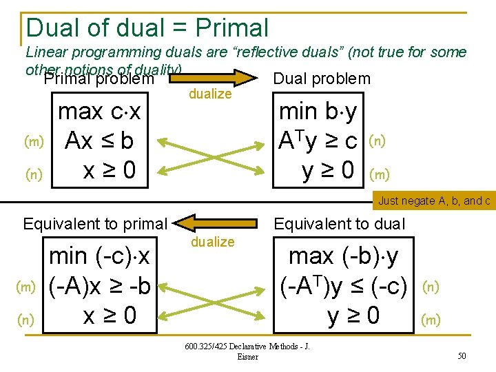
Dual of dual = Primal Linear programming duals are “reflective duals” (not true for some other notions of duality) Primal problem (m) (n) max c x Ax ≤ b x≥ 0 dualize Dual problem min b y A Ty ≥ c y≥ 0 (n) (m) Just negate A, b, and c Equivalent to primal (m) (n) min (-c) x (-A)x ≥ -b x≥ 0 Equivalent to dualize max (-b) y (-AT)y ≤ (-c) y≥ 0 600. 325/425 Declarative Methods - J. Eisner (n) (m) 50

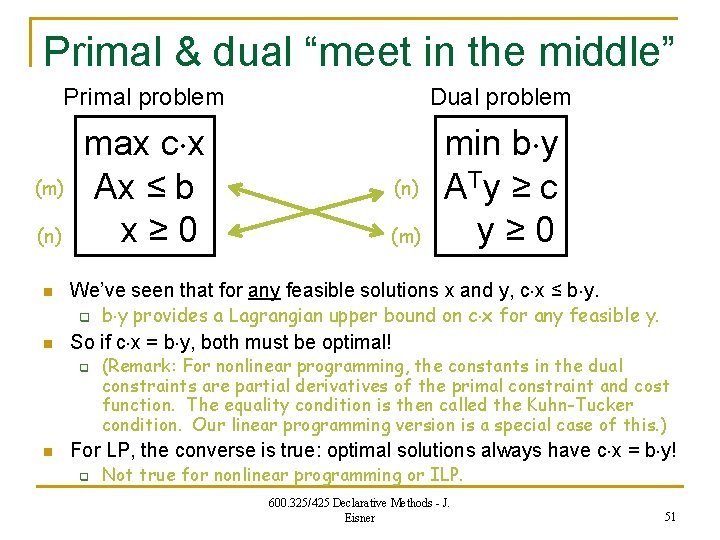
Primal & dual “meet in the middle” Primal problem Dual problem max c x Ax ≤ b x≥ 0 min b y A Ty ≥ c y≥ 0 (m) (n) n b y provides a Lagrangian upper bound on c x for any feasible y. So if c x = b y, both must be optimal! q n (m) We’ve seen that for any feasible solutions x and y, c x ≤ b y. q n (n) (Remark: For nonlinear programming, the constants in the dual constraints are partial derivatives of the primal constraint and cost function. The equality condition is then called the Kuhn-Tucker condition. Our linear programming version is a special case of this. ) For LP, the converse is true: optimal solutions always have c x = b y! q Not true for nonlinear programming or ILP. 600. 325/425 Declarative Methods - J. Eisner 51

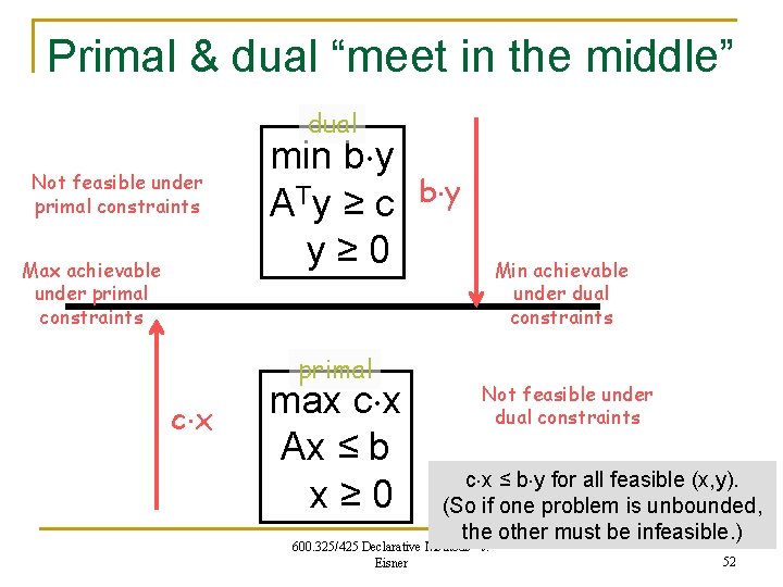
Primal & dual “meet in the middle” dual Not feasible under primal constraints Max achievable under primal constraints min b y A Ty ≥ c y≥ 0 primal c x max c x Ax ≤ b x≥ 0 b y Min achievable under dual constraints Not feasible under dual constraints c x ≤ b y for all feasible (x, y). (So if one problem is unbounded, the other must be infeasible. ) 600. 325/425 Declarative Methods - J. Eisner 52

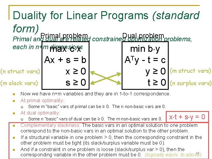
Duality for Linear Programs (standard form) Primal problem Dual problem Primal and dual are related constrained optimization problems, each in n+m max dimensions c x min b y (n struct vars) (m slack vars) n n (m struct vars) (n surplus vars) Some m “basic” vars of primal can be ≥ 0. The n non-basic vars are 0. At dual optimality: q n A Ty - t = c y≥ 0 t≥ 0 Now we have n+m variables and they are in 1 -to-1 correspondence. At primal optimality: q n Ax + s = b x≥ 0 s≥ 0 Some n “basic” vars of dual can be ≥ 0. The m non-basic vars are 0. x t + s y = 0 Complementary slackness: The basic vars in an optimal solution to one problem correspond to the non-basic vars in an optimal solution to the other problem. If a structural variable in one problem > 0, then the corresponding constraint in the other problem must be tight (its slack/surplus variable must be 0). And if a constraint in one problem is loose (slack/surplus var > 0), then the 53 corresponding variable in the other problem must be 0. (logically equiv. to above)

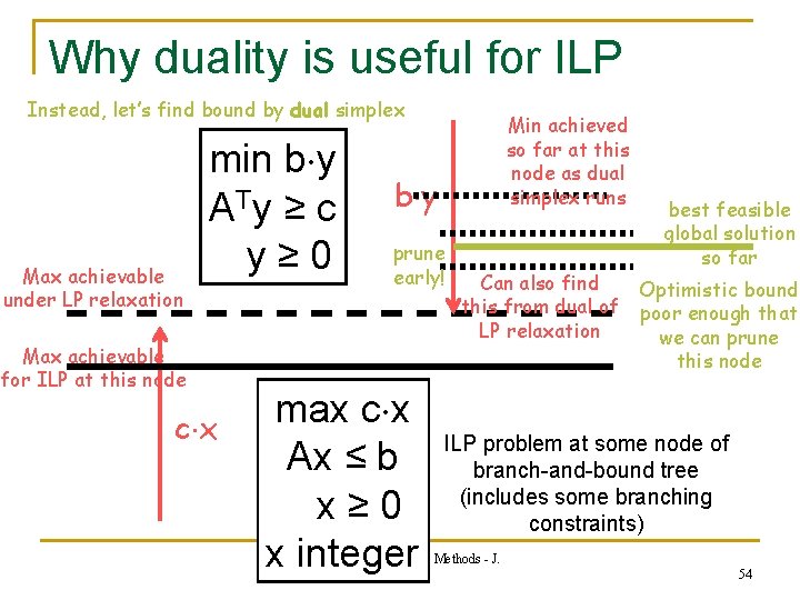
Why duality is useful for ILP Instead, let’s find bound by dual simplex Max achievable under LP relaxation min b y A Ty ≥ c y≥ 0 Max achievable for ILP at this node c x Min achieved so far at this node as dual simplex runs b y prune early! max c x Ax ≤ b x≥ 0 x integer Can also find this from dual of LP relaxation best feasible global solution so far Optimistic bound poor enough that we can prune this node ILP problem at some node of branch-and-bound tree (includes some branching constraints) 600. 325/425 Declarative Methods - J. Eisner 54

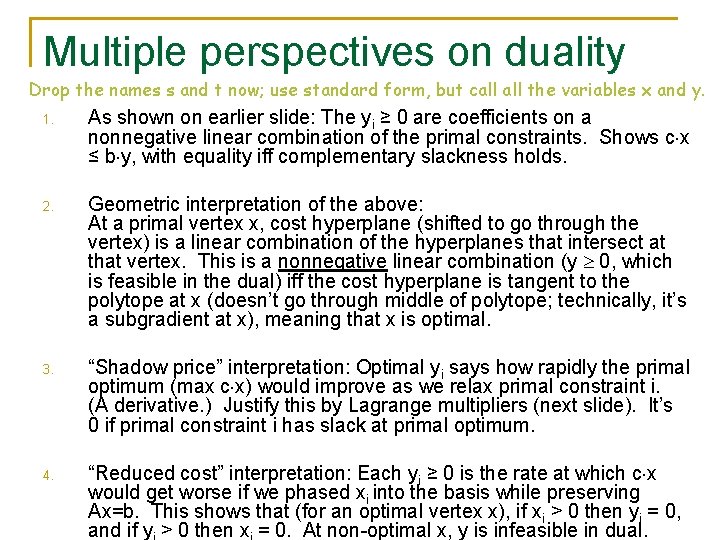
Multiple perspectives on duality Drop the names s and t now; use standard form, but call the variables x and y. 1. As shown on earlier slide: The yi ≥ 0 are coefficients on a nonnegative linear combination of the primal constraints. Shows c x ≤ b y, with equality iff complementary slackness holds. 2. Geometric interpretation of the above: At a primal vertex x, cost hyperplane (shifted to go through the vertex) is a linear combination of the hyperplanes that intersect at that vertex. This is a nonnegative linear combination (y 0, which is feasible in the dual) iff the cost hyperplane is tangent to the polytope at x (doesn’t go through middle of polytope; technically, it’s a subgradient at x), meaning that x is optimal. 3. “Shadow price” interpretation: Optimal yi says how rapidly the primal optimum (max c x) would improve as we relax primal constraint i. (A derivative. ) Justify this by Lagrange multipliers (next slide). It’s 0 if primal constraint i has slack at primal optimum. 4. “Reduced cost” interpretation: Each yi ≥ 0 is the rate at which c x would get worse if we phased xi into the basis while preserving Ax=b. This shows that (for an optimal vertex x), if xi > 0 then yi = 0, and if y > 0 then x = 0. At non-optimal x, y is infeasible in dual.

Where Does Duality Come From? n More generally, let’s look at Lagrangian relaxation. max c(x) subject to a(x) ≤ b (let x* denote the solution) Technically, this is not the method of Lagrange multipliers. Lagrange (18 th century) only handled equality constraints. Karush (1939) and Kuhn & Tucker (1951) generalized to inequalities.

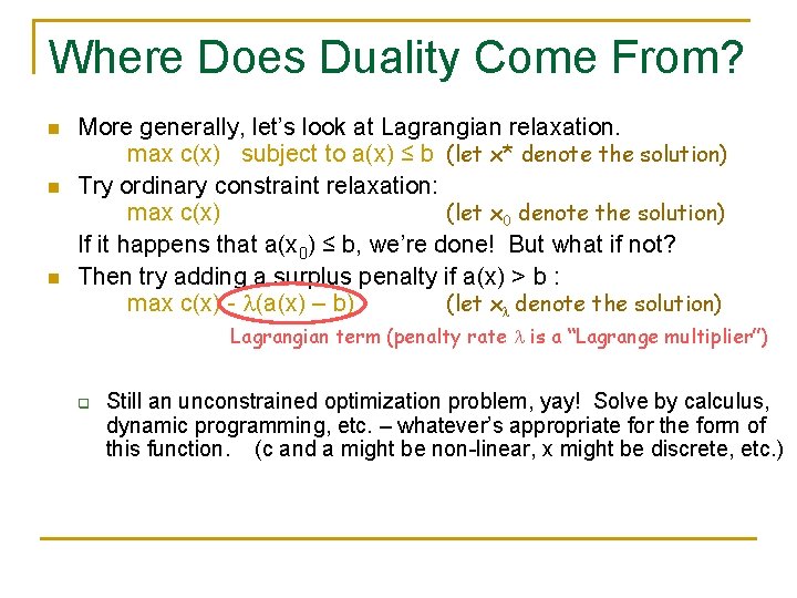
Where Does Duality Come From? n n n More generally, let’s look at Lagrangian relaxation. max c(x) subject to a(x) ≤ b (let x* denote the solution) Try ordinary constraint relaxation: max c(x) (let x 0 denote the solution) If it happens that a(x 0) ≤ b, we’re done! But what if not? Then try adding a surplus penalty if a(x) > b : max c(x) - (a(x) – b) (let x denote the solution) Lagrangian term (penalty rate is a “Lagrange multiplier”) q Still an unconstrained optimization problem, yay! Solve by calculus, dynamic programming, etc. – whatever’s appropriate for the form of this function. (c and a might be non-linear, x might be discrete, etc. )

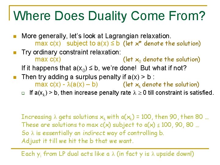
Where Does Duality Come From? n n n More generally, let’s look at Lagrangian relaxation. max c(x) subject to a(x) ≤ b (let x* denote the solution) Try ordinary constraint relaxation: max c(x) (let x 0 denote the solution) If it happens that a(x 0) ≤ b, we’re done! But what if not? Then try adding a surplus penalty if a(x) > b : max c(x) - (a(x) – b) (let x denote the solution) q If a(x ) > b, then increase penalty rate 0 till constraint is satisfied. Increasing gets solutions x with a(x ) = 100, then 90, then 80 … These are solutions to max c(x) subject to a(x) ≤ 100, 90, 80 … So is essentially an indirect way of controlling b. Adjust it till we hit the b that we want. Each yi from LP dual acts like a (in fact y is upside down!)

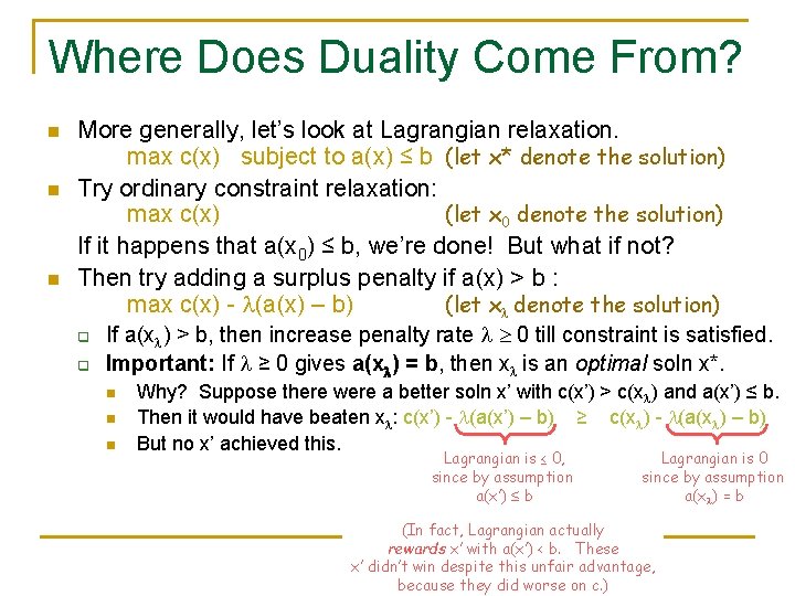
Where Does Duality Come From? n n n More generally, let’s look at Lagrangian relaxation. max c(x) subject to a(x) ≤ b (let x* denote the solution) Try ordinary constraint relaxation: max c(x) (let x 0 denote the solution) If it happens that a(x 0) ≤ b, we’re done! But what if not? Then try adding a surplus penalty if a(x) > b : max c(x) - (a(x) – b) (let x denote the solution) q q If a(x ) > b, then increase penalty rate 0 till constraint is satisfied. Important: If ≥ 0 gives a(x ) = b, then x is an optimal soln x*. n n n Why? Suppose there were a better soln x’ with c(x’) > c(x ) and a(x’) ≤ b. Then it would have beaten x : c(x’) - (a(x’) – b) ≥ c(x ) - (a(x ) – b) But no x’ achieved this. Lagrangian is ≤ 0, since by assumption a(x’) ≤ b Lagrangian is 0 since by assumption a(x ) = b (In fact, Lagrangian actually rewards x’ with a(x’) < b. These x’ didn’t win despite this unfair advantage, because they did worse on c. )

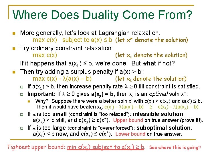
Where Does Duality Come From? n n n More generally, let’s look at Lagrangian relaxation. max c(x) subject to a(x) ≤ b (let x* denote the solution) Try ordinary constraint relaxation: max c(x) (let x 0 denote the solution) If it happens that a(x 0) ≤ b, we’re done! But what if not? Then try adding a surplus penalty if a(x) > b : max c(x) - (a(x) – b) (let x denote the solution) q q If a(x ) > b, then increase penalty rate 0 till constraint is satisfied. Important: If ≥ 0 gives a(x ) = b, then x is an optimal soln x*. Why? Suppose there were a better soln x’ with c(x’) > c(x ) and a(x’) ≤ b. Then it would have beaten x : c(x’) - (a(x’) – b) ≥ c(x ) - (a(x ) – b) If is too small (constraint is “too relaxed”): infeasible solution. a(x ) > b still, and c(x ) ≥ c(x*). Upper bound on true answer (prove it!). If is too large (constraint is “overenforced”): suboptimal solution. a(x ) < b now, and c(x ) ≤ c(x*). Lower bound on true answer. n q q Tightest upper bound: min c(x ) subject to a(x ) ≥ b. See where this is going?

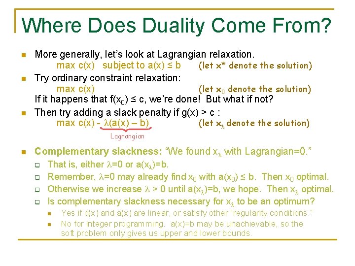
Where Does Duality Come From? n n n More generally, let’s look at Lagrangian relaxation. max c(x) subject to a(x) ≤ b (let x* denote the solution) Try ordinary constraint relaxation: max c(x) (let x 0 denote the solution) If it happens that f(x 0) ≤ c, we’re done! But what if not? Then try adding a slack penalty if g(x) > c : max c(x) - (a(x) – b) (let x denote the solution) Lagrangian n Complementary slackness: “We found x with Lagrangian=0. ” q q That is, either =0 or a(x )=b. Remember, =0 may already find x 0 with a(x 0) ≤ b. Then x 0 optimal. Otherwise we increase > 0 until a(x )=b, we hope. Then x optimal. Is complementary slackness necessary for x to be an optimum? n n Yes if c(x) and a(x) are linear, or satisfy other “regularity conditions. ” No for integer programming. a(x)=b may be unachievable, so the soft problem only gives us upper and lower bounds.

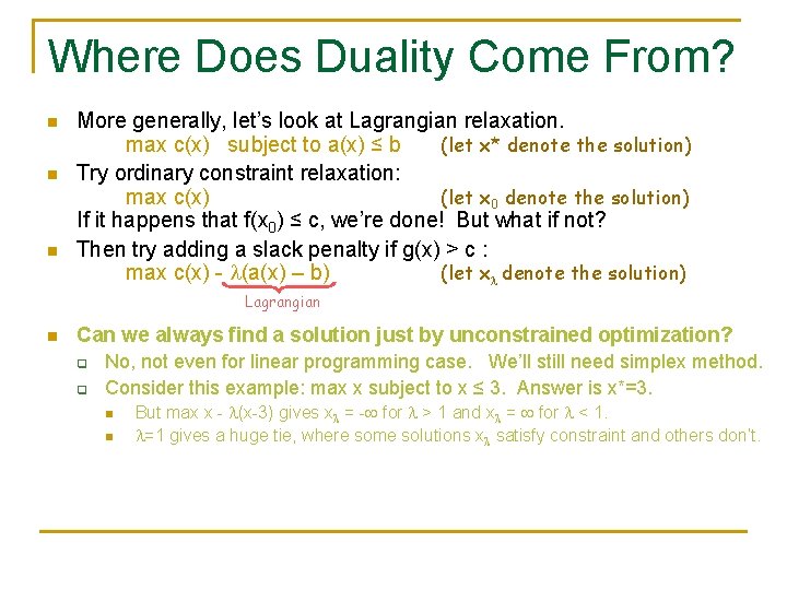
Where Does Duality Come From? n n n More generally, let’s look at Lagrangian relaxation. max c(x) subject to a(x) ≤ b (let x* denote the solution) Try ordinary constraint relaxation: max c(x) (let x 0 denote the solution) If it happens that f(x 0) ≤ c, we’re done! But what if not? Then try adding a slack penalty if g(x) > c : max c(x) - (a(x) – b) (let x denote the solution) Lagrangian n Can we always find a solution just by unconstrained optimization? q q No, not even for linear programming case. We’ll still need simplex method. Consider this example: max x subject to x ≤ 3. Answer is x*=3. n n But max x - (x-3) gives x = - for > 1 and x = for < 1. =1 gives a huge tie, where some solutions x satisfy constraint and others don’t.

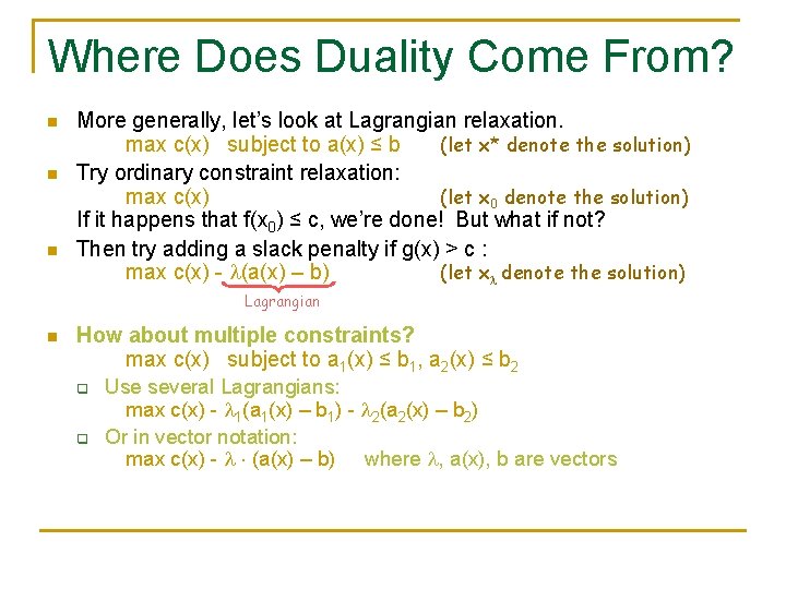
Where Does Duality Come From? n n n More generally, let’s look at Lagrangian relaxation. max c(x) subject to a(x) ≤ b (let x* denote the solution) Try ordinary constraint relaxation: max c(x) (let x 0 denote the solution) If it happens that f(x 0) ≤ c, we’re done! But what if not? Then try adding a slack penalty if g(x) > c : max c(x) - (a(x) – b) (let x denote the solution) Lagrangian n How about multiple constraints? max c(x) subject to a 1(x) ≤ b 1, a 2(x) ≤ b 2 q q Use several Lagrangians: max c(x) - 1(a 1(x) – b 1) - 2(a 2(x) – b 2) Or in vector notation: max c(x) - (a(x) – b) where , a(x), b are vectors