Linear Programming Models 1 Introduction to Linear Programming

線性規劃模式 Linear Programming Models 1

線性規劃簡介 Introduction to Linear Programming • 線性規劃模型(Linear Programming model)是在一組 「線性」的限制式(a set of linear constraints)之下， 尋找極大化(maximize)或極小化(minimize)一個特 定的目標函數(objective function) • 線性規劃模型由下列三個部分組成: – 一組決策變數 (A set of decision variables) – 一個特定的目標函數(An objective function) – 一組「線性」的限制式 (A set of constraints) 2

典型範例 The Galaxy Industries Production Problem • Galaxy 生產兩種玩具模型: – 宇宙光Space Ray. – 射擊手Zapper. • 資源限制(Resources) – 1000 磅特殊塑膠化合物 (special plastic) – 每週 40 小時生產時間(40 hrs of production time per week) 6

典型範例 The Galaxy Industries Production Problem • 市場需求(Marketing requirement) – 每週總產量至多 700 打 – Space Rays週產量不能過Zappers 350打以 上 • 技術係數 (Technological inputs) (Table 2. 2) – Space Rays 每打需要 2 pounds 塑膠與 3分 鐘生產時間 – Zappers每打需要 1 pound 塑膠與 4分鐘生產 7 時間

典型範例 The Galaxy Industries Production Problem • 生產需求: – Space Ray每打利潤(profit) $8，Zappers每打 利潤(profit) $5 – 盡量多生產Space Ray，剩餘資源再生產 Zapper • 目前生產計畫: Space Rays = 450 dozen 8(450) + 5(100) Zapper = 100 dozen Profit = $4100 per week 8

管理是尋求一個生產排程 為了是能增加公司的利潤 Management is seeking a production schedule that will increase the company’s profit. 9

線性規劃模式可以提供一種深 入與聰明之方法來解決此問題 A linear programming model can provide an insight and an intelligent solution to this problem. 10

典型範例線性規劃模式 The Galaxy Linear Programming Model • 決策變數(Decisions variables): – X 1 = 每週生產的 Space Rays 打數 – X 2 =每週生產的 Zappers 打數 • 目標函數(Objective Function): – 極大化每週總利潤 11

典型範例線性規劃模式 The Galaxy Linear Programming Model Max 8 X 1 + 5 X 2 (每週總利潤) subject to 2 X 1 + 1 X 2 £ 1000 (塑膠原料, Plastic) 3 X 1 + 4 X 2 £ 2400 (生產時間, Production Time) X 1 + X 2 £ 700 (最大產量, Total production) X 1 - X 2 £ 350 (組合) 12

線性規劃模式圖形分析 Graphical Analysis of Linear Programming 滿足模型全部限制式的所有點集合稱為 The set of all points that satisfy all the constraints of the model is called a 可行區域 FEASIBLE REGION 13

圖形表示法(graphical presentation) ―所有限制式(all the constraints) ―目標函數(objective function) ―可行點(three types of feasible points) 14

圖形分析 – 可行區域 Graphical Analysis – the Feasible Region X 2 The non-negativity constraints (非負限制式) X 1 15

圖形分析 – 可行區域 Graphical Analysis – the Feasible Region X 2 Plastic限制式 2 X 1+X 2 £ 1000 700 Total production 限制式 X 1+X 2 £ 700 (多餘) 500 Infeasible Production Time 限制式 3 X 1+4 X 2 £ 2400 Feasible 500 700 X 1 16

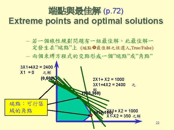
圖形分析 – 可行區域 (p. 67~68) Graphical Analysis – the Feasible Region X 2 Plastic限制式 2 X 1+X 2 £ 1000 700 Total production 限制式 X 1+X 2 £ 700 (多餘) 500 Infeasible Mix限制式 Production Time 限制式 3 X 1+4 X 2£ 2400 X 1 -X 2 £ 350 Feasible 500 700 內部點Interior points. 邊界點 Boundary points. • 可行點(feasible points)有三種 X 1 端點Extreme point 17

以圖形求解是為了尋求最佳解 Solving Graphically for an Optimal Solution 18

尋求最佳解圖解程序 (p. 71) The search for an optimal solution X 2 1000 700 由任一個 profit開始, say profit = $1, 250. 往利潤增加方向移動 increase the profit, if poss 持續平行移動到無法增加為止 continue until it becomes infeasible 500 Optimal Profit =$4360 紅色線段 Profit =$1250 X 1 500 19

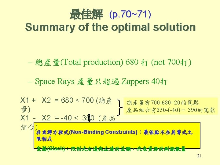
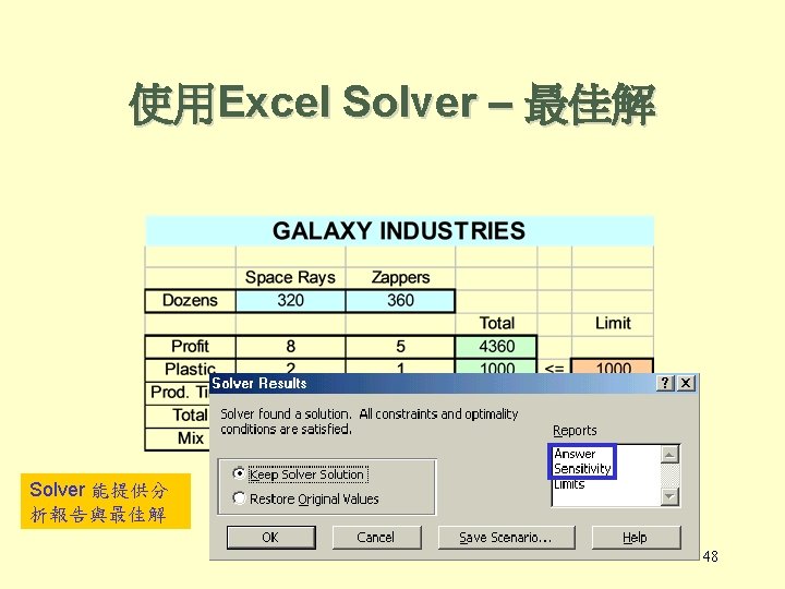
最佳解 (p. 69) Summary of the optimal solution Space Rays X 1 * = 320 dozen Zappers X 2 * = 360 dozen. Excel試算表 Profit Z * = $4360 – 此最佳解使用了所有的塑膠原料(plastic)與生產時間 (production hours). 2 X 1 + 1 X 2 = 1000 (塑膠原料, Plastic) 3 X 1 + 4 X 2 = 2400 (生產時間, Production Time) 束縛方程式(Binding Constraints): 等式被滿足之限制 式 20

目標函數係數之敏感性分析 Sensitivity Analysis of Objective Function Coefficients. 1000 M 1 + 5 X 2 佳解為(0, 600) 最佳解仍為 (320, 360) 8 X C 1係數=2，最 ax 600 減少C 1係數 由 8→ 3. 75 M ax x 3 4 X. 75 1 + X 5 X 2 (0, 600) 2 Ma X 2 (320, 360)Max 2 X 1 + 5 X 而(320, 360)不 再是最佳解 2 X 1 500 800 26

1000 目標函數係數之敏感性分析 Sensitivity Analysis of Objective Function Coefficients. X 2 8 X ax M 1 增加C 1係數，由 8→ 10 最佳解仍包含(320, 360) + 5 X 1 + 5 (320, 360) X X 2 5 X +5 3. 7 1 Ma x 0 X x 1 Ma 2 600 2 C 1係數的最佳範圍: [3. 75, 10] 同理，C 2係數的最佳範圍: [4, 10. 67] (Can you find it ? ) 400 600 800 X 1 27

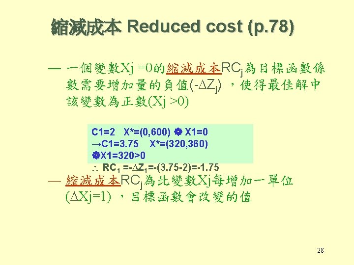
目標函數係數之敏感性分析 縮減成本 (p. 79) X 2 1000 ∆X 1=1 (由 X 1=0→X 1=1) X 1 ≥ 1 Ma x 3 . 75 X 1 +5 X ∆Z=2998. 25 -3000 = 1. 75 RC 1 =-1. 75 (1, 599. 25) Z=2998. 25 2 (0, 600) Z=3000 600 Max 2 X 1 + 5 X 2 X 1 500 800 29

影子價格Shadow Price – 圖形表示 graphical demonstration Plastic限制 式 X 2 1000 2 X 1 0) 最佳解由 Z*= X*$4360 =(320. 8, 359. 4)(320, 360)→(320. 8, 359. 4 Z* = $4363. 4 ) 01 10 <= 00 x 2 10 +1 <= x 2 +1 2 X 1 500 X*=(320, 36 Productio n time 限制式 當右手值增加(例如 由 1000→ 1001)則可 行區域擴大 Shadow price = 4363. 40 – 4360. 00 = 3. 40 X 1 500 33

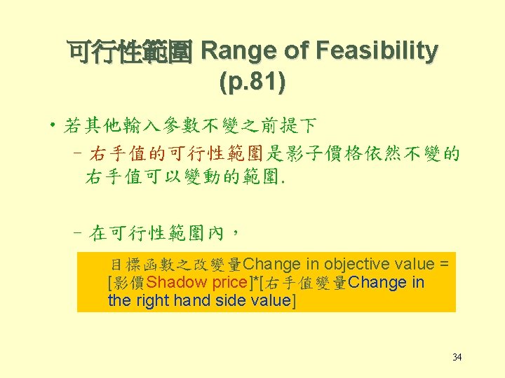
塑膠的可行性範圍 Range of Feasibility (p. 81) Plastic限制式 X 2 2 X 1 塑膠原料的數量可以增加到一個 新限制式成為Binding為止 x 2 +1 1000 00 10 <= Total Production限 制式 X 1 + X 2 £ 700 500 Total Production成為 新的束縛限制式 (New Binding Constraint) Production time 限制式 此處為不可行解 X 1 500 35

Plastic 塑膠的可行性範圍 Range of Feasibility 限制式 X 2 2 X 1 +1 1000 x 2 0 00 £ 1 Total Production 限制式 X 1+X 2 ≤ 700 請注意看： 當塑膠數量增加時最佳解的變化 塑膠的可行性範圍 上限 = 2 X 1 + 1 X 2 =2*(400)+300=1100 600 X 1+ X 2 = 700 3 X 1+4 X 2 = 2400 之解 X*=(400, 300)為 最佳解 Production time 限制式 3 X 1+4 X 2 ≤ 2400 500 X 1 36

塑膠的可行性範圍 Range of Feasibility X 2 Infeasible 1000 solution 600 X 1 = 0成為 0 新的束縛限制式 3 X 1+ 4 X 2 = 2400 X 1 = 0 之解 X*=(0, 600)為最佳 解 請注意看： 當塑膠數量減少時最佳解的變化 Plastic 限制式 2 X 1 + 1 X 2 £ 1000 塑膠的可行性範圍 下限 =2 X 1 + 1 X 2 = 2*(0)+1*600=600 500 Production time 限制式 3 X 1+4 X 2 ≤ 2400 X 1 37

(3) 其他後最佳性變動 (p. 84) Other Post - Optimality Changes • 加入一個新限制式(Addition of a constraint) 決定最佳解是否滿足此限制式 Yes, the solution is still optimal No, re-solve the problem (the new objective function is worse than the original one) • 刪除一個限制式(Deletion of a constraint) 決定刪除的限制式是否為束縛限制式 • Yes, re-solve the problem (the new objective function is better than the original one) • No, the solution is still optimal 40

其他後最佳性變動 (p. 84) Other Post - Optimality Changes • 刪除變數 (Deletion of a variable) 決定被刪除變數在最佳解中是否為 0 Yes, the solution is still optimal No, re-solve the problem (the new objective function is worse than the original one) • 增加變數 (Addition of a variable)─考慮淨邊際利潤(Net Marginal Profit) 41

其他後最佳性變動 (p. 85) Other Post - Optimality Changes • 左手係數的變動(Changes in the left - hand side coefficients. ) 43

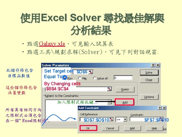
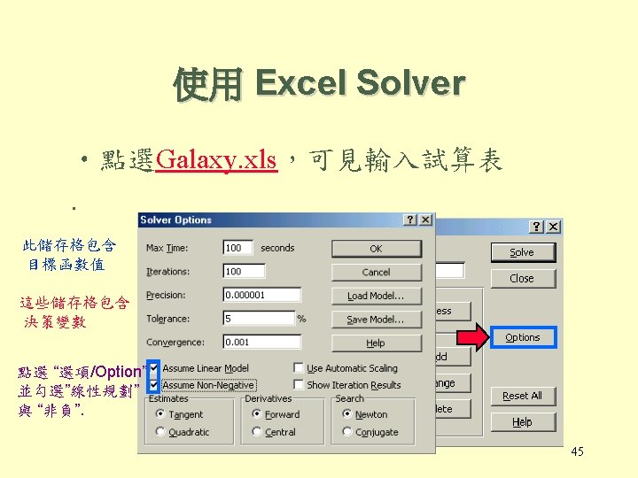
使用 Excel Solver • 點選Galaxy. xls，可見輸入試算表 按Solve以求最佳 解 Set Target cell Equal To: $D$ 6 By Changing $B$4: $C$ cells 4 $D$7: $D$10<=$F$7: $F$10 46

使用Excel Solver – 最佳解 47

使用Excel Solver –解答報表 Answer Report 49

使用Excel Solver –敏感性分析報 表Sensitivity Report 50

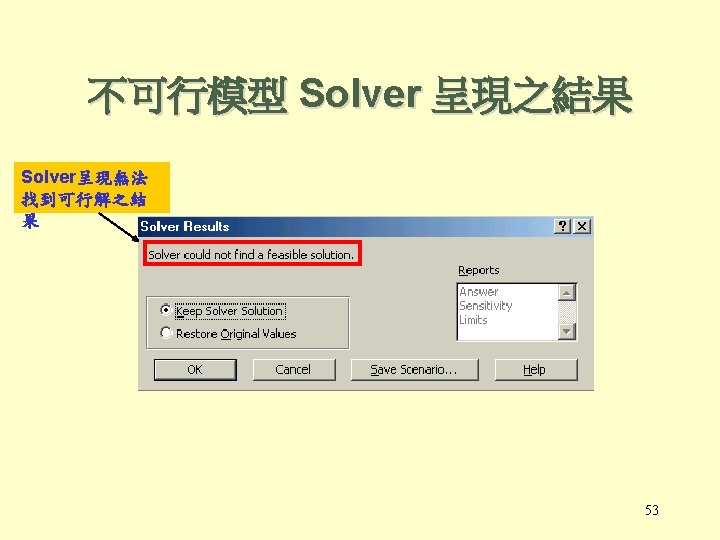
不可行模型 Infeasible Model No point, simultaneously, 1 lies both above line and below lines 2 2 and 3 . 3 1 52

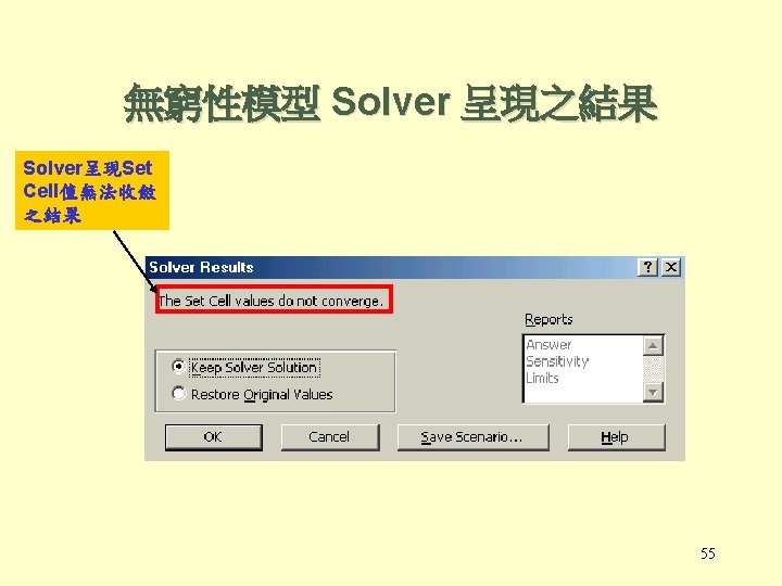
無窮性 Unbounded solution Ma 目 標 函 數 可 行 xim ize 區 域 54

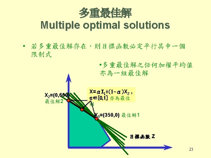
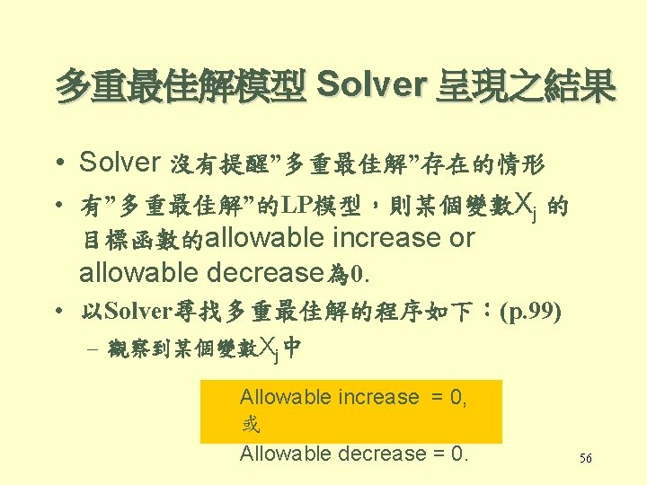
多重最佳解模型 Solver 呈現之結果 • 加入一個限制式: Objective function = Current optimal value. – If Allowable increase = 0, change the objective to Maximize Xj – If Allowable decrease = 0, change the objective to Minimize Xj Excel試算表 57