7 SUPPLEMENT Capacity and Constraint Management Power Point

7 SUPPLEMENT Capacity and Constraint Management Power. Point presentation to accompany Heizer and Render Operations Management, Eleventh Edition Principles of Operations Management, Ninth Edition Power. Point slides by Jeff Heyl © 2014 Pearson Education, Inc. © 2014 Pearson Education, S 7 - 1

Outline ► ► Capacity Bottleneck Analysis and the Theory of Constraints Break-Even Analysis Reducing Risk with Incremental Changes © 2014 Pearson Education, Inc. S 7 - 2

Outline - Continued ► ► Applying Expected Monetary Value (EMV) to Capacity Decisions Applying Investment Analysis to Strategy-Driven Investments © 2014 Pearson Education, Inc. S 7 - 3

Learning Objectives When you complete this supplement you should be able to : 1. Define capacity 2. Determine design capacity, effective capacity, and utilization 3. Perform bottleneck analysis 4. Compute break-even © 2014 Pearson Education, Inc. S 7 - 4

Learning Objectives When you complete this supplement you should be able to : 5. Determine the expected monetary value of a capacity decision 6. Compute net present value © 2014 Pearson Education, Inc. S 7 - 5

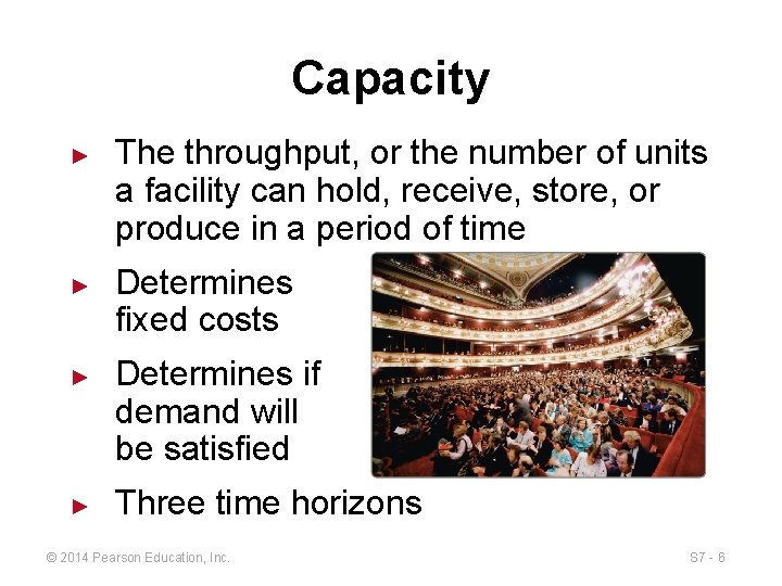
Capacity ► ► The throughput, or the number of units a facility can hold, receive, store, or produce in a period of time Determines fixed costs Determines if demand will be satisfied Three time horizons © 2014 Pearson Education, Inc. S 7 - 6

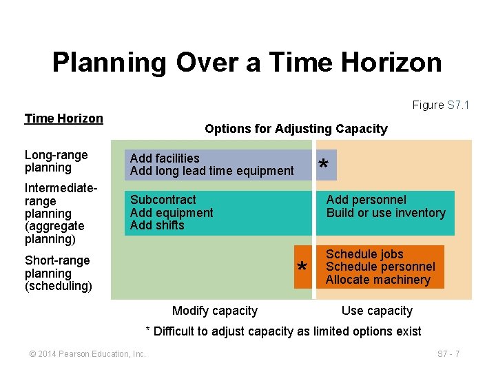
Planning Over a Time Horizon Figure S 7. 1 Time Horizon Options for Adjusting Capacity Long-range planning Add facilities Add long lead time equipment Intermediaterange planning (aggregate planning) Subcontract Add equipment Add shifts Short-range planning (scheduling) * Add personnel Build or use inventory * Modify capacity Schedule jobs Schedule personnel Allocate machinery Use capacity * Difficult to adjust capacity as limited options exist © 2014 Pearson Education, Inc. S 7 - 7

Design and Effective Capacity ► Design capacity is the maximum theoretical output of a system ► ► Normally expressed as a rate Effective capacity is the capacity a firm expects to achieve given current operating constraints ► Often lower than design capacity © 2014 Pearson Education, Inc. S 7 - 8

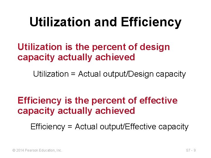
Utilization and Efficiency Utilization is the percent of design capacity actually achieved Utilization = Actual output/Design capacity Efficiency is the percent of effective capacity actually achieved Efficiency = Actual output/Effective capacity © 2014 Pearson Education, Inc. S 7 - 9

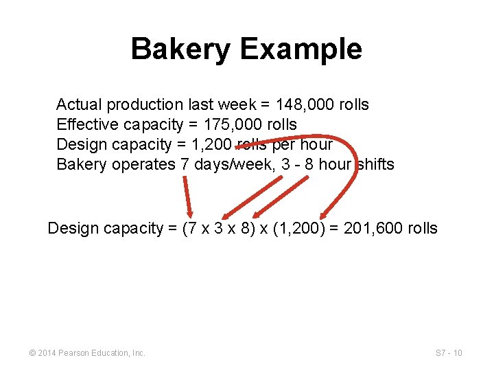
Bakery Example Actual production last week = 148, 000 rolls Effective capacity = 175, 000 rolls Design capacity = 1, 200 rolls per hour Bakery operates 7 days/week, 3 - 8 hour shifts Design capacity = (7 x 3 x 8) x (1, 200) = 201, 600 rolls © 2014 Pearson Education, Inc. S 7 - 10

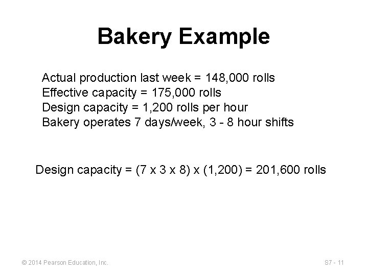
Bakery Example Actual production last week = 148, 000 rolls Effective capacity = 175, 000 rolls Design capacity = 1, 200 rolls per hour Bakery operates 7 days/week, 3 - 8 hour shifts Design capacity = (7 x 3 x 8) x (1, 200) = 201, 600 rolls © 2014 Pearson Education, Inc. S 7 - 11

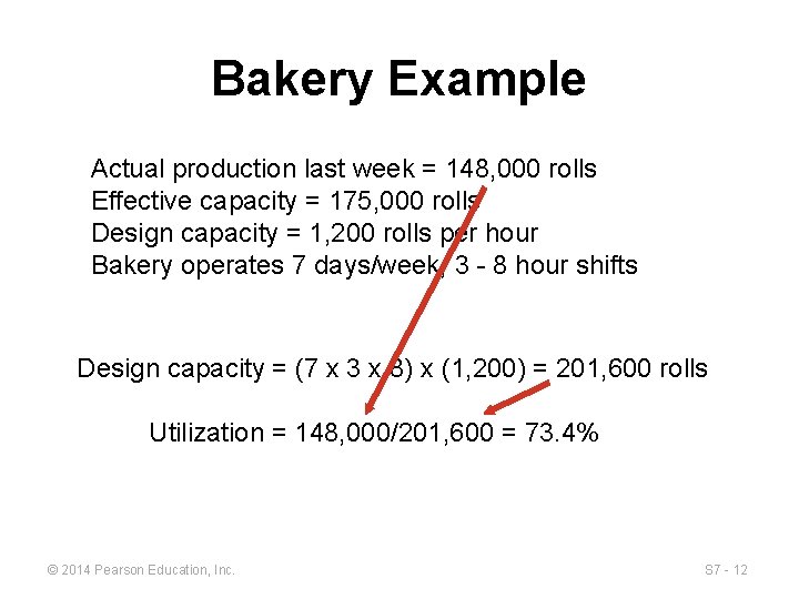
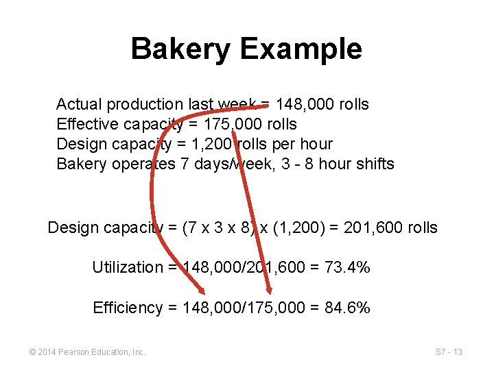
Bakery Example Actual production last week = 148, 000 rolls Effective capacity = 175, 000 rolls Design capacity = 1, 200 rolls per hour Bakery operates 7 days/week, 3 - 8 hour shifts Design capacity = (7 x 3 x 8) x (1, 200) = 201, 600 rolls Utilization = 148, 000/201, 600 = 73. 4% © 2014 Pearson Education, Inc. S 7 - 12

Bakery Example Actual production last week = 148, 000 rolls Effective capacity = 175, 000 rolls Design capacity = 1, 200 rolls per hour Bakery operates 7 days/week, 3 - 8 hour shifts Design capacity = (7 x 3 x 8) x (1, 200) = 201, 600 rolls Utilization = 148, 000/201, 600 = 73. 4% Efficiency = 148, 000/175, 000 = 84. 6% © 2014 Pearson Education, Inc. S 7 - 13

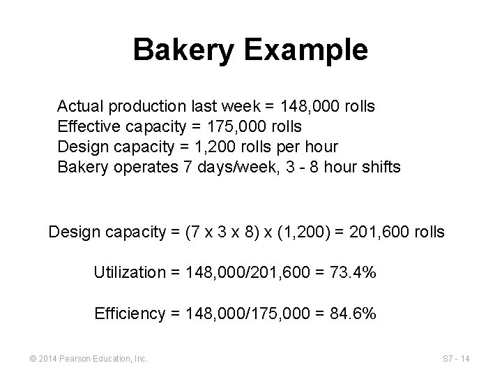
Bakery Example Actual production last week = 148, 000 rolls Effective capacity = 175, 000 rolls Design capacity = 1, 200 rolls per hour Bakery operates 7 days/week, 3 - 8 hour shifts Design capacity = (7 x 3 x 8) x (1, 200) = 201, 600 rolls Utilization = 148, 000/201, 600 = 73. 4% Efficiency = 148, 000/175, 000 = 84. 6% © 2014 Pearson Education, Inc. S 7 - 14

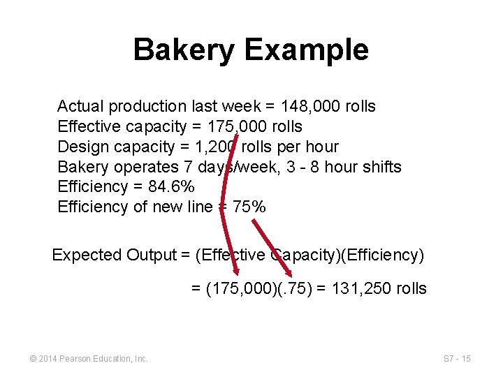
Bakery Example Actual production last week = 148, 000 rolls Effective capacity = 175, 000 rolls Design capacity = 1, 200 rolls per hour Bakery operates 7 days/week, 3 - 8 hour shifts Efficiency = 84. 6% Efficiency of new line = 75% Expected Output = (Effective Capacity)(Efficiency) = (175, 000)(. 75) = 131, 250 rolls © 2014 Pearson Education, Inc. S 7 - 15

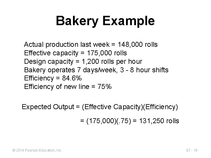
Bakery Example Actual production last week = 148, 000 rolls Effective capacity = 175, 000 rolls Design capacity = 1, 200 rolls per hour Bakery operates 7 days/week, 3 - 8 hour shifts Efficiency = 84. 6% Efficiency of new line = 75% Expected Output = (Effective Capacity)(Efficiency) = (175, 000)(. 75) = 131, 250 rolls © 2014 Pearson Education, Inc. S 7 - 16

Capacity and Strategy ► ► Capacity decisions impact all 10 decisions of operations management as well as other functional areas of the organization Capacity decisions must be integrated into the organization’s mission and strategy © 2014 Pearson Education, Inc. S 7 - 17

Capacity Considerations 1. Forecast demand accurately 2. Match technology increments and sales volume 3. Find the optimum operating size (volume) 4. Build for change © 2014 Pearson Education, Inc. S 7 - 18

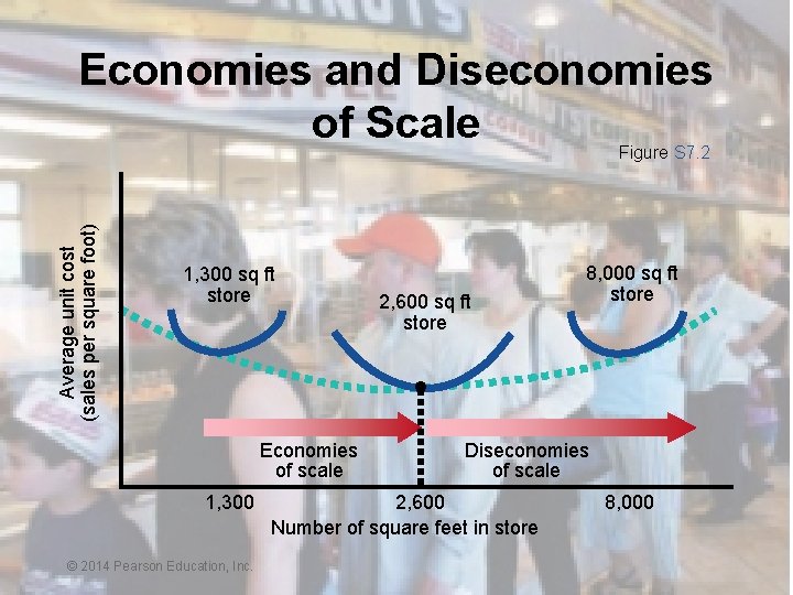
Economies and Diseconomies of Scale Average unit cost (sales per square foot) Figure S 7. 2 1, 300 sq ft store Economies of scale 1, 300 © 2014 Pearson Education, Inc. © 2014 Pearson Education, 2, 600 sq ft store 8, 000 sq ft store Diseconomies of scale 2, 600 Number of square feet in store 8, 000 S 7 - 19

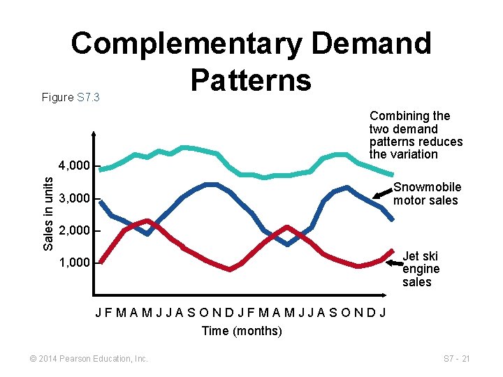
Managing Demand ► Demand exceeds capacity ► ► Curtail demand by raising prices, scheduling longer lead time Long term solution is to increase capacity Capacity exceeds demand ► Stimulate market ► Product changes Adjusting to seasonal demands ► Produce products with complementary demand patterns © 2014 Pearson Education, Inc. S 7 - 20

Complementary Demand Patterns Figure S 7. 3 Sales in units 4, 000 – Combining the two demand patterns reduces the variation 3, 000 – Snowmobile motor sales 2, 000 – 1, 000 – Jet ski engine sales JFMAMJJASONDJ Time (months) © 2014 Pearson Education, Inc. S 7 - 21

Tactics for Matching Capacity to Demand 1. Making staffing changes 2. Adjusting equipment ► Purchasing additional machinery ► Selling or leasing out existing equipment 3. Improving processes to increase throughput 4. Redesigning products to facilitate more throughput 5. Adding process flexibility to meet changing product preferences 6. Closing facilities © 2014 Pearson Education, Inc. S 7 - 22

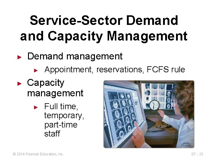
Service-Sector Demand Capacity Management ► Demand management ► ► Appointment, reservations, FCFS rule Capacity management ► Full time, temporary, part-time staff © 2014 Pearson Education, Inc. S 7 - 23

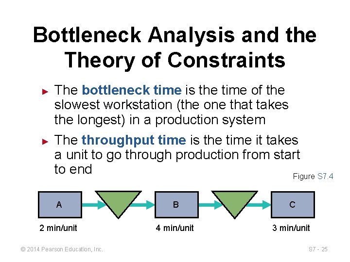
Bottleneck Analysis and the Theory of Constraints ► ► Each work area can have its own unique capacity Capacity analysis determines the throughput capacity of workstations in a system A bottleneck is a limiting factor or constraint A bottleneck has the lowest effective capacity in a system © 2014 Pearson Education, Inc. S 7 - 24

Bottleneck Analysis and the Theory of Constraints ► ► The bottleneck time is the time of the slowest workstation (the one that takes the longest) in a production system The throughput time is the time it takes a unit to go through production from start to end Figure S 7. 4 A B C 2 min/unit 4 min/unit 3 min/unit © 2014 Pearson Education, Inc. S 7 - 25

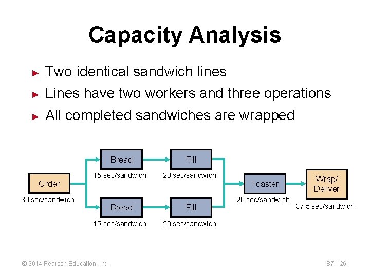
Capacity Analysis ► Two identical sandwich lines ► Lines have two workers and three operations ► All completed sandwiches are wrapped Order Bread Fill 15 sec/sandwich 20 sec/sandwich 30 sec/sandwich Bread Fill 15 sec/sandwich 20 sec/sandwich © 2014 Pearson Education, Inc. Toaster 20 sec/sandwich Wrap/ Deliver 37. 5 sec/sandwich S 7 - 26

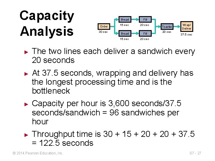
Capacity Analysis ► ► Order 30 sec Bread Fill 15 sec 20 sec Wrap/ Deliver Toaster 20 sec 37. 5 sec The two lines each deliver a sandwich every 20 seconds At 37. 5 seconds, wrapping and delivery has the longest processing time and is the bottleneck Capacity per hour is 3, 600 seconds/37. 5 seconds/sandwich = 96 sandwiches per hour Throughput time is 30 + 15 + 20 + 37. 5 = 122. 5 seconds © 2014 Pearson Education, Inc. S 7 - 27

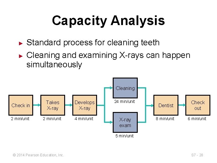
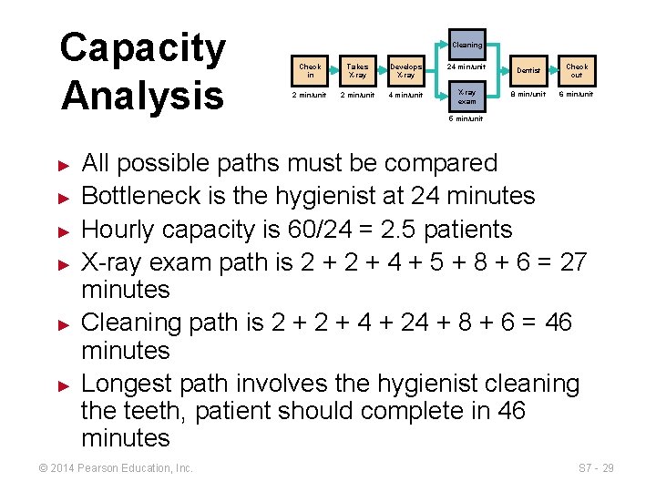
Capacity Analysis ► ► Standard process for cleaning teeth Cleaning and examining X-rays can happen simultaneously Cleaning Check in Takes X-ray Develops X-ray 24 min/unit 2 min/unit 4 min/unit X-ray exam Dentist Check out 8 min/unit 6 min/unit 5 min/unit © 2014 Pearson Education, Inc. S 7 - 28

Capacity Analysis ► ► ► Cleaning Check in Takes X-ray Develops X-ray 24 min/unit 2 min/unit 4 min/unit X-ray exam Dentist Check out 8 min/unit 6 min/unit 5 min/unit All possible paths must be compared Bottleneck is the hygienist at 24 minutes Hourly capacity is 60/24 = 2. 5 patients X-ray exam path is 2 + 4 + 5 + 8 + 6 = 27 minutes Cleaning path is 2 + 4 + 24 + 8 + 6 = 46 minutes Longest path involves the hygienist cleaning the teeth, patient should complete in 46 minutes © 2014 Pearson Education, Inc. S 7 - 29

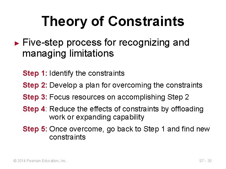
Theory of Constraints ► Five-step process for recognizing and managing limitations Step 1: Identify the constraints Step 2: Develop a plan for overcoming the constraints Step 3: Focus resources on accomplishing Step 2 Step 4: Reduce the effects of constraints by offloading work or expanding capability Step 5: Once overcome, go back to Step 1 and find new constraints © 2014 Pearson Education, Inc. S 7 - 30

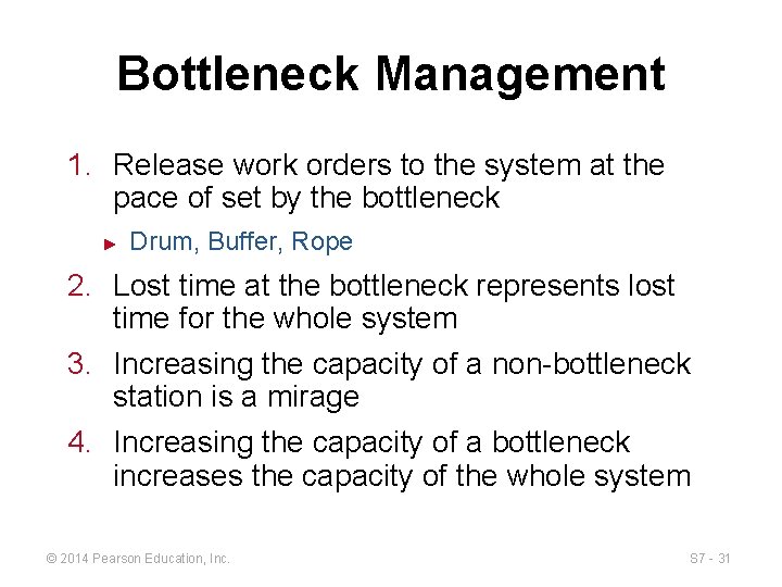
Bottleneck Management 1. Release work orders to the system at the pace of set by the bottleneck ► Drum, Buffer, Rope 2. Lost time at the bottleneck represents lost time for the whole system 3. Increasing the capacity of a non-bottleneck station is a mirage 4. Increasing the capacity of a bottleneck increases the capacity of the whole system © 2014 Pearson Education, Inc. S 7 - 31

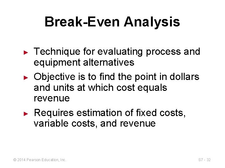
Break-Even Analysis ► ► ► Technique for evaluating process and equipment alternatives Objective is to find the point in dollars and units at which cost equals revenue Requires estimation of fixed costs, variable costs, and revenue © 2014 Pearson Education, Inc. S 7 - 32

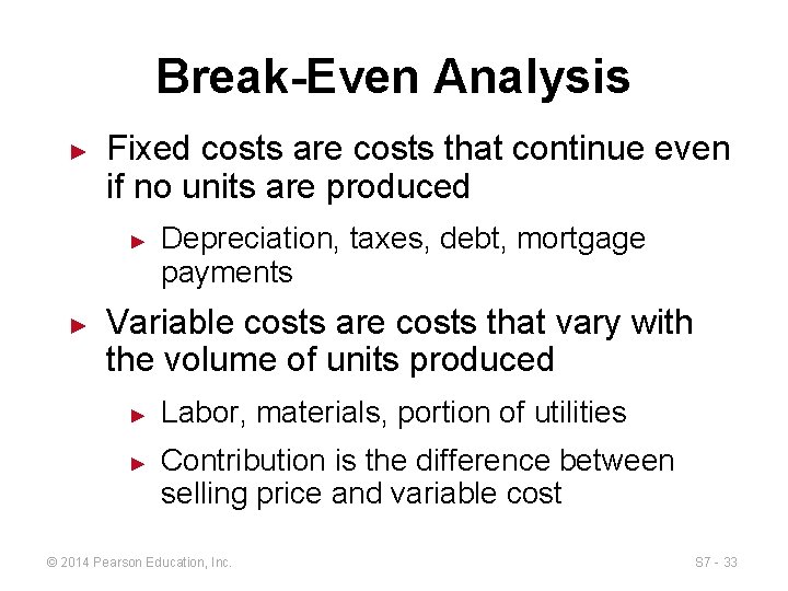
Break-Even Analysis ► Fixed costs are costs that continue even if no units are produced ► ► Depreciation, taxes, debt, mortgage payments Variable costs are costs that vary with the volume of units produced ► ► Labor, materials, portion of utilities Contribution is the difference between selling price and variable cost © 2014 Pearson Education, Inc. S 7 - 33

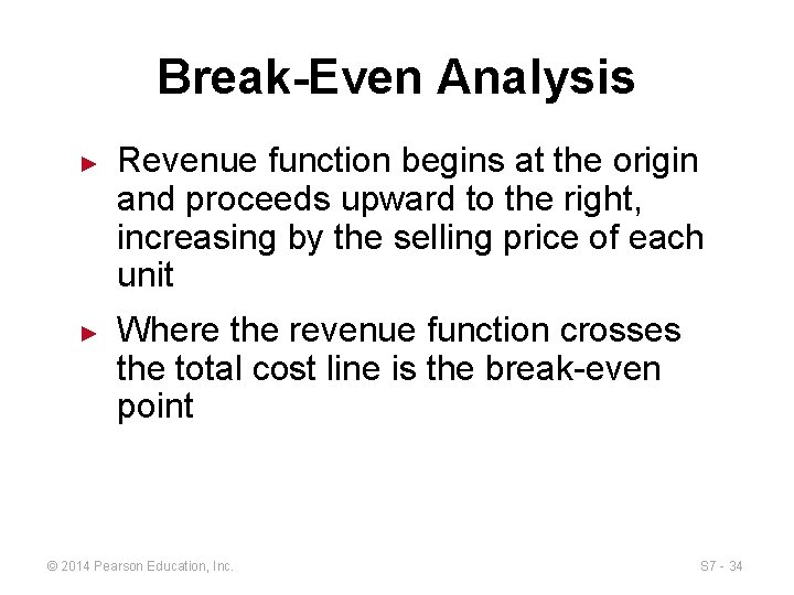
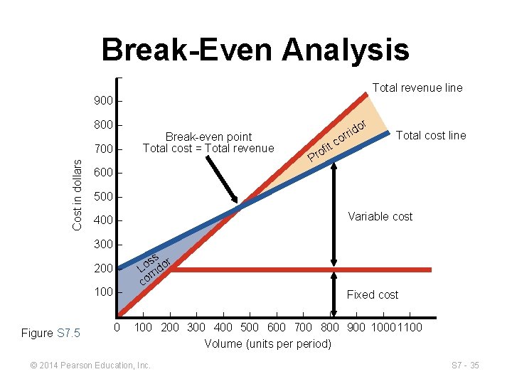
Break-Even Analysis ► ► Revenue function begins at the origin and proceeds upward to the right, increasing by the selling price of each unit Where the revenue function crosses the total cost line is the break-even point © 2014 Pearson Education, Inc. S 7 - 34

Break-Even Analysis – Total revenue line 900 – 800 – Cost in dollars 700 – r Break-even point Total cost = Total revenue o d i r r o it c Total cost line of r P 600 – 500 – Variable cost 400 – 300 – 200 – 100 – ss or o L rid r co Fixed cost | | | – 0 100 200 300 400 500 600 700 800 900 10001100 Volume (units period) | Figure S 7. 5 © 2014 Pearson Education, Inc. S 7 - 35

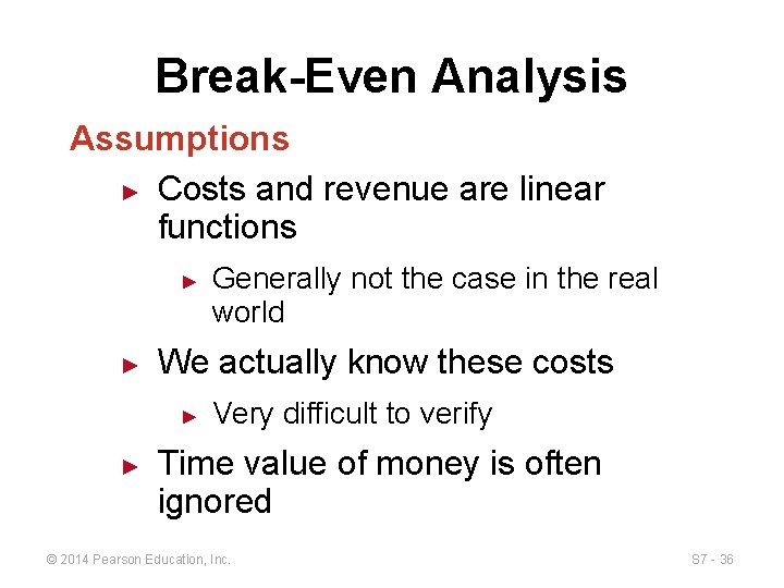
Break-Even Analysis Assumptions ► Costs and revenue are linear functions ► ► We actually know these costs ► ► Generally not the case in the real world Very difficult to verify Time value of money is often ignored © 2014 Pearson Education, Inc. S 7 - 36

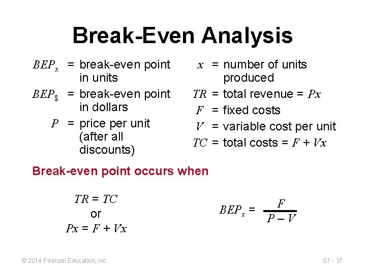
Break-Even Analysis BEPx = break-even point in units BEP$ = break-even point in dollars P = price per unit (after all discounts) x = number of units produced TR = total revenue = Px F = fixed costs V = variable cost per unit TC = total costs = F + Vx Break-even point occurs when TR = TC or Px = F + Vx © 2014 Pearson Education, Inc. BEPx = F P–V S 7 - 37

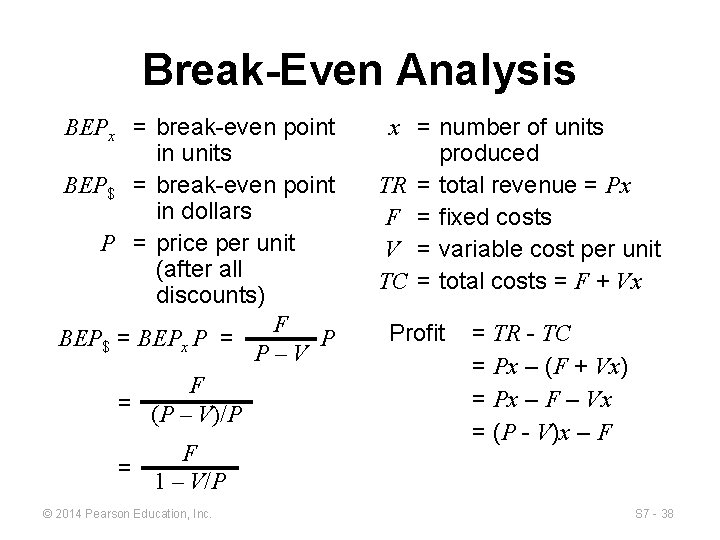
Break-Even Analysis BEPx = break-even point in units BEP$ = break-even point in dollars P = price per unit (after all discounts) F BEP$ = BEPx P = P P–V F = (P – V)/P = F 1 – V/P © 2014 Pearson Education, Inc. x = number of units produced TR = total revenue = Px F = fixed costs V = variable cost per unit TC = total costs = F + Vx Profit = TR - TC = Px – (F + Vx) = Px – F – Vx = (P - V)x – F S 7 - 38

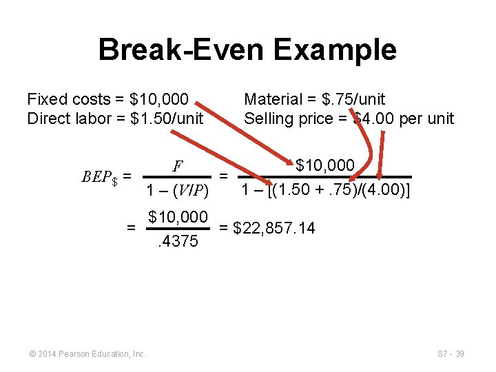
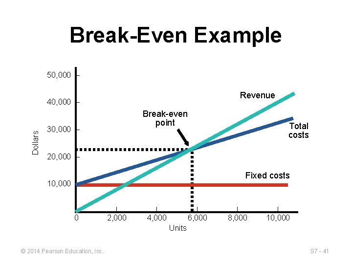
Break-Even Example Fixed costs = $10, 000 Direct labor = $1. 50/unit BEP$ = Material = $. 75/unit Selling price = $4. 00 per unit $10, 000 F = 1 – [(1. 50 +. 75)/(4. 00)] 1 – (V/P) $10, 000 = = $22, 857. 14. 4375 © 2014 Pearson Education, Inc. S 7 - 39

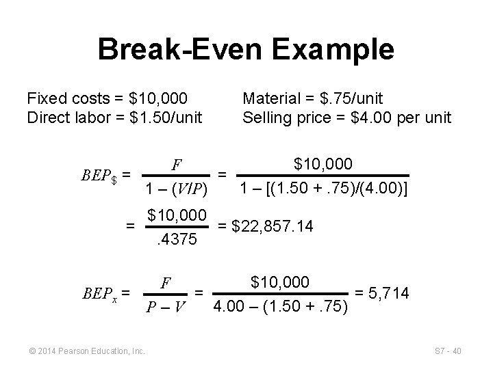
Break-Even Example Fixed costs = $10, 000 Direct labor = $1. 50/unit BEP$ = Material = $. 75/unit Selling price = $4. 00 per unit $10, 000 F = 1 – [(1. 50 +. 75)/(4. 00)] 1 – (V/P) $10, 000 = = $22, 857. 14. 4375 $10, 000 F BEPx = = = 5, 714 4. 00 – (1. 50 +. 75) P–V © 2014 Pearson Education, Inc. S 7 - 40

Break-Even Example 50, 000 – Revenue Dollars 40, 000 – Break-even point 30, 000 – Total costs 20, 000 – Fixed costs 10, 000 – | – 0 | | | 2, 000 4, 000 6, 000 8, 000 10, 000 Units © 2014 Pearson Education, Inc. S 7 - 41

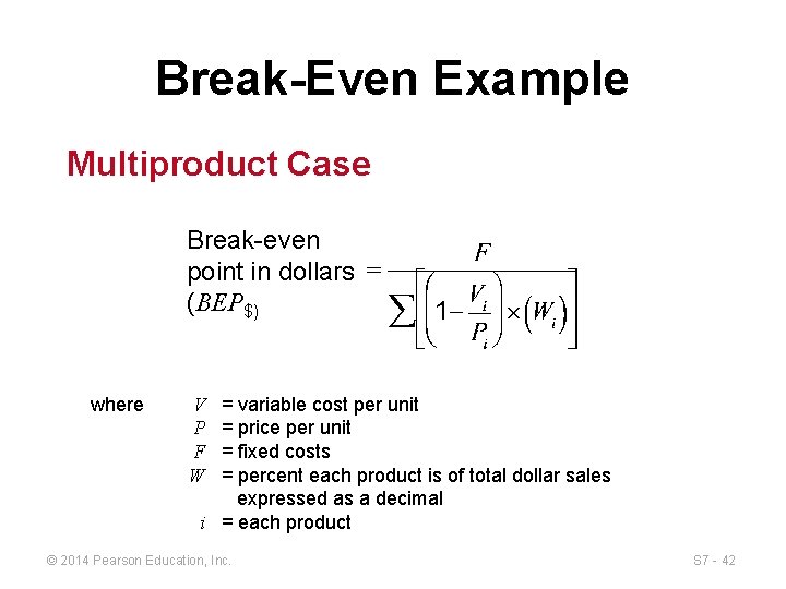
Break-Even Example Multiproduct Case Break-even point in dollars (BEP$) where = variable cost per unit = price per unit = fixed costs = percent each product is of total dollar sales expressed as a decimal i = each product V P F W © 2014 Pearson Education, Inc. S 7 - 42

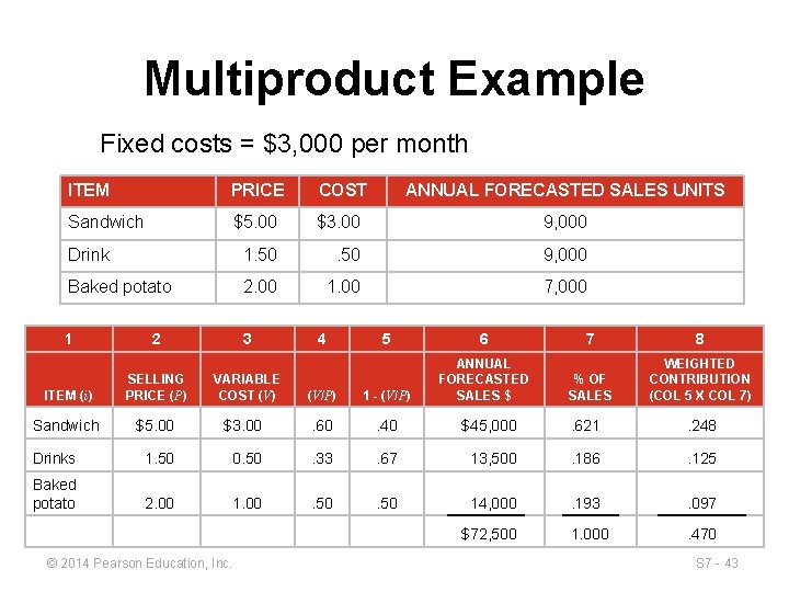
Multiproduct Example Fixed costs = $3, 000 per month ITEM PRICE COST ANNUAL FORECASTED SALES UNITS Sandwich $5. 00 $3. 00 9, 000 Drink 1. 50 9, 000 Baked potato 2. 00 1. 00 7, 000 1 3 2 VARIABLE COST (V) 4 5 6 (V/P) 1 - (V/P) ANNUAL FORECASTED SALES $ 7 8 % OF SALES WEIGHTED CONTRIBUTION (COL 5 X COL 7) ITEM (i) SELLING PRICE (P) Sandwich $5. 00 $3. 00 . 60 . 40 $45, 000 . 621 . 248 Drinks 1. 50 0. 50 . 33 . 67 13, 500 . 186 . 125 Baked potato 2. 00 1. 00 . 50 14, 000 . 193 . 097 $72, 500 1. 000 . 470 © 2014 Pearson Education, Inc. S 7 - 43

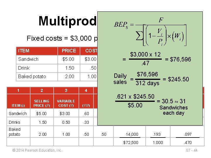
Multiproduct Example Fixed costs = $3, 000 per month ITEM PRICE COST Sandwich $5. 00 $3. 00 Drink 1. 50 Baked potato 2. 00 1 3 2 ITEM (i) SELLING PRICE (P) Sandwich $5. 00 Drinks Baked potato VARIABLE COST (V) 4 ANNUAL FORECASTED SALES UNITS $3, 000 x 12 9, 000 = = $76, 596. 47 9, 000 $76, 596 Daily 7, 000 = sales 312 days = $245. 50 5 6 7 8 ANNUAL WEIGHTED. 621 x $245. 50 %= OF 30. 5 CONTRIBUTION FORECASTED 31 SALES $ SALES (COL 5 X COL 7) $5. 00 Sandwiches (V/P) 1 - (V/P) $3. 00 . 60 . 40 $45, 000 . 621 each day. 248 1. 50 0. 50 . 33 . 67 13, 500 . 186 . 125 2. 00 1. 00 . 50 14, 000 . 193 . 097 $72, 500 1. 000 . 470 © 2014 Pearson Education, Inc. S 7 - 44

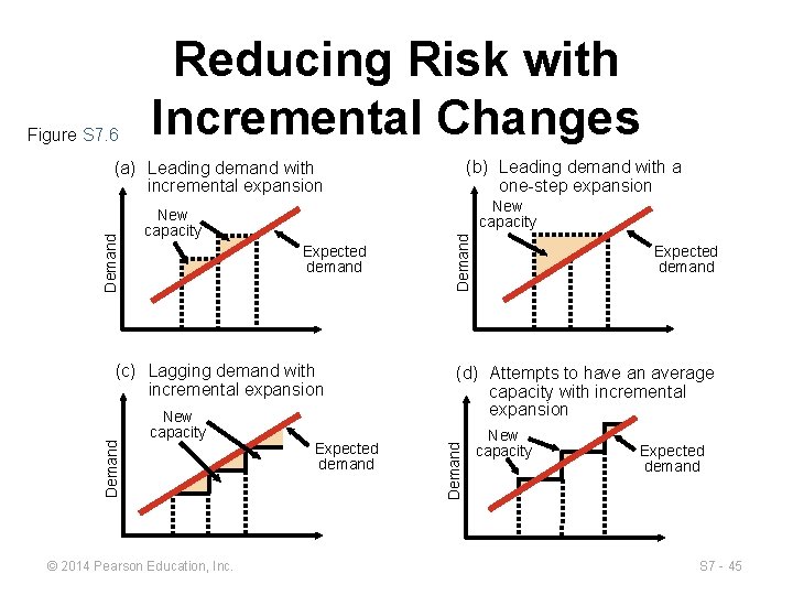
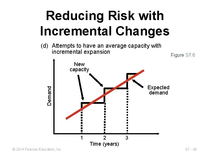
Figure S 7. 6 Reducing Risk with Incremental Changes (b) Leading demand with a one-step expansion Expected demand Demand (c) Lagging demand with incremental expansion New capacity © 2014 Pearson Education, Inc. Expected demand Demand New capacity Expected demand (d) Attempts to have an average capacity with incremental expansion Demand (a) Leading demand with incremental expansion New capacity Expected demand S 7 - 45

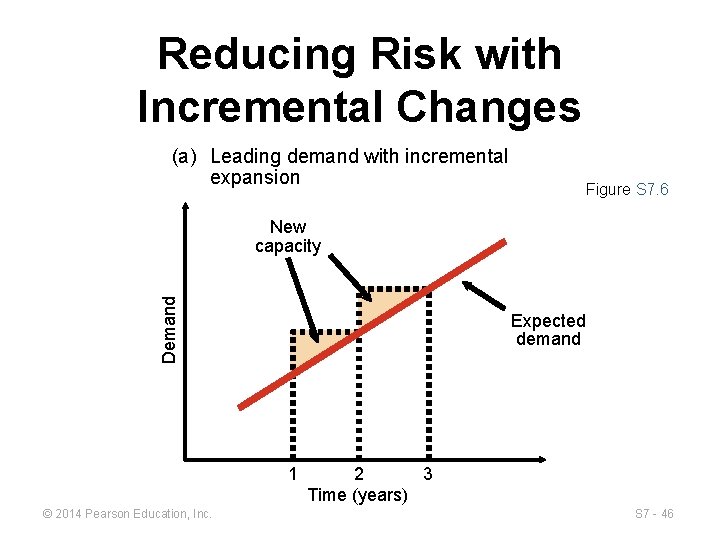
Reducing Risk with Incremental Changes (a) Leading demand with incremental expansion Figure S 7. 6 Demand New capacity Expected demand 1 © 2014 Pearson Education, Inc. 2 3 Time (years) S 7 - 46

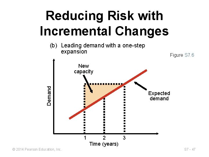
Reducing Risk with Incremental Changes (b) Leading demand with a one-step expansion Figure S 7. 6 Demand New capacity Expected demand 1 © 2014 Pearson Education, Inc. 2 3 Time (years) S 7 - 47

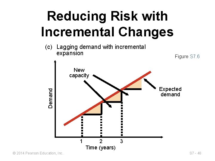
Reducing Risk with Incremental Changes (c) Lagging demand with incremental expansion Figure S 7. 6 New capacity Demand Expected demand 1 © 2014 Pearson Education, Inc. 2 3 Time (years) S 7 - 48

Reducing Risk with Incremental Changes (d) Attempts to have an average capacity with incremental expansion Figure S 7. 6 New capacity Demand Expected demand 1 © 2014 Pearson Education, Inc. 2 Time (years) 3 S 7 - 49

Applying Expected Monetary Value (EMV) and Capacity Decisions ► ► Determine states of nature ► Future demand ► Market favorability Assign probability values to states of nature to determine expected value © 2014 Pearson Education, Inc. S 7 - 50

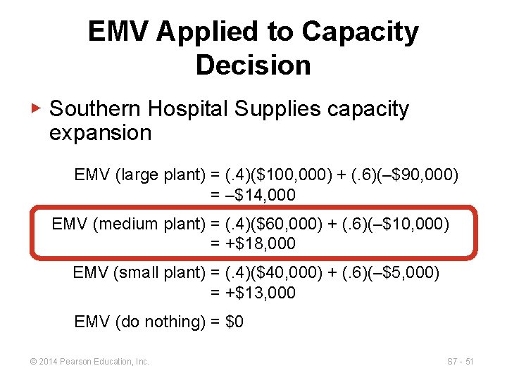
EMV Applied to Capacity Decision ▶ Southern Hospital Supplies capacity expansion EMV (large plant) = (. 4)($100, 000) + (. 6)(–$90, 000) = –$14, 000 EMV (medium plant) = (. 4)($60, 000) + (. 6)(–$10, 000) = +$18, 000 EMV (small plant) = (. 4)($40, 000) + (. 6)(–$5, 000) = +$13, 000 EMV (do nothing) = $0 © 2014 Pearson Education, Inc. S 7 - 51

Strategy-Driven Investment ► ► Operations managers may have to decide among various financial options Analyzing capacity alternatives should include capital investment, variable cost, cash flows, and net present value © 2014 Pearson Education, Inc. S 7 - 52

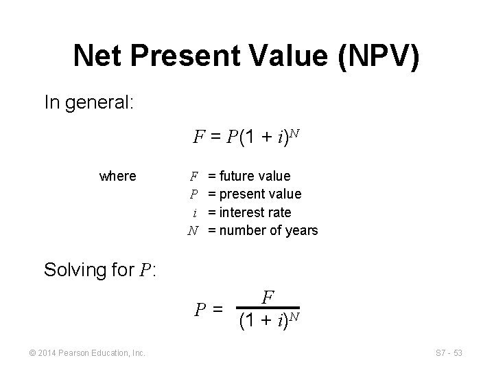
Net Present Value (NPV) In general: F = P(1 + i)N where F P i N = future value = present value = interest rate = number of years Solving for P: F P= (1 + i)N © 2014 Pearson Education, Inc. S 7 - 53

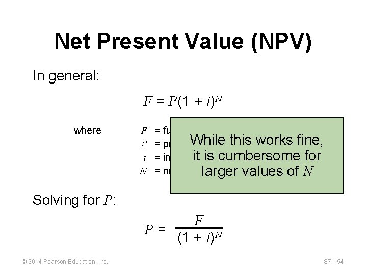
Net Present Value (NPV) In general: F = P(1 + i)N where F P i N = future value While = present value this works fine, is cumbersome for = interestitrate = number of years values of N larger Solving for P: F P= (1 + i)N © 2014 Pearson Education, Inc. S 7 - 54

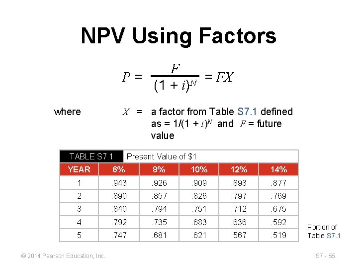
NPV Using Factors F P= = FX N (1 + i) where X = a factor from Table S 7. 1 defined as = 1/(1 + i)N and F = future value TABLE S 7. 1 Present Value of $1 YEAR 6% 8% 10% 12% 14% 1 . 943 . 926 . 909 . 893 . 877 2 . 890 . 857 . 826 . 797 . 769 3 . 840 . 794 . 751 . 712 . 675 4 . 792 . 735 . 683 . 636 . 592 5 . 747 . 681 . 621 . 567 . 519 © 2014 Pearson Education, Inc. Portion of Table S 7. 1 S 7 - 55

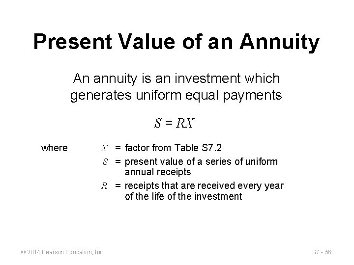
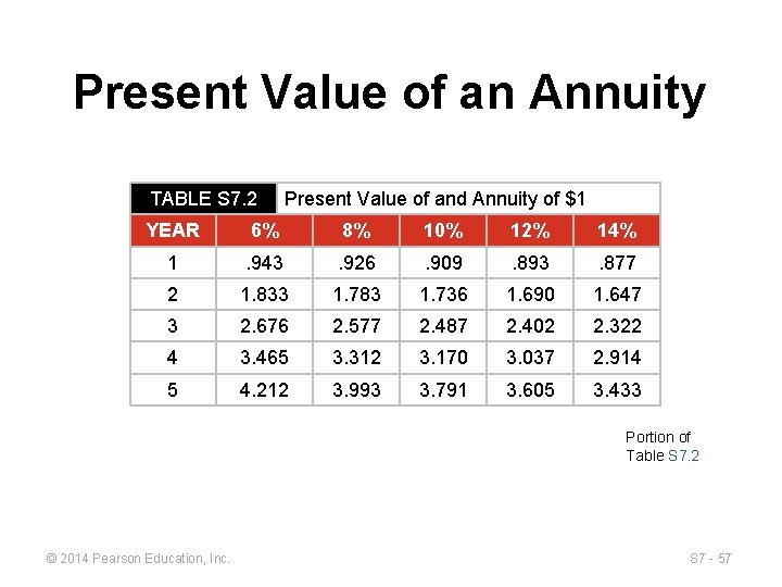
Present Value of an Annuity An annuity is an investment which generates uniform equal payments S = RX where X = factor from Table S 7. 2 S = present value of a series of uniform annual receipts R = receipts that are received every year of the life of the investment © 2014 Pearson Education, Inc. S 7 - 56

Present Value of an Annuity TABLE S 7. 2 Present Value of and Annuity of $1 YEAR 6% 8% 10% 12% 14% 1 . 943 . 926 . 909 . 893 . 877 2 1. 833 1. 783 1. 736 1. 690 1. 647 3 2. 676 2. 577 2. 487 2. 402 2. 322 4 3. 465 3. 312 3. 170 3. 037 2. 914 5 4. 212 3. 993 3. 791 3. 605 3. 433 Portion of Table S 7. 2 © 2014 Pearson Education, Inc. S 7 - 57

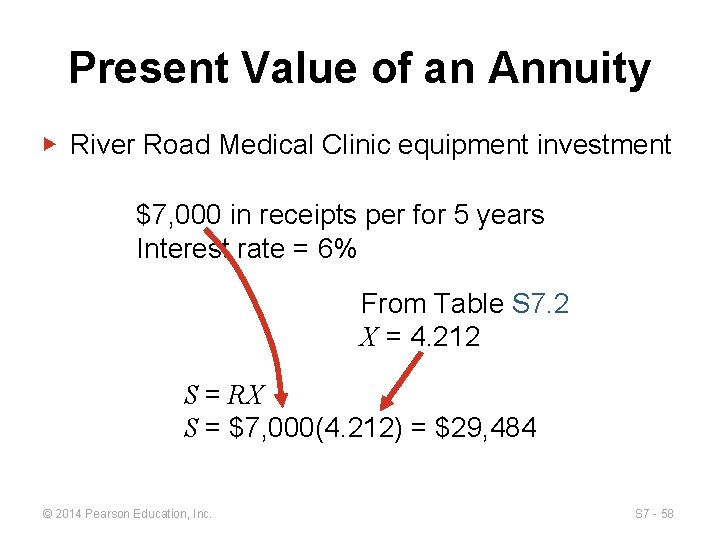
Present Value of an Annuity ▶ River Road Medical Clinic equipment investment $7, 000 in receipts per for 5 years Interest rate = 6% From Table S 7. 2 X = 4. 212 S = RX S = $7, 000(4. 212) = $29, 484 © 2014 Pearson Education, Inc. S 7 - 58

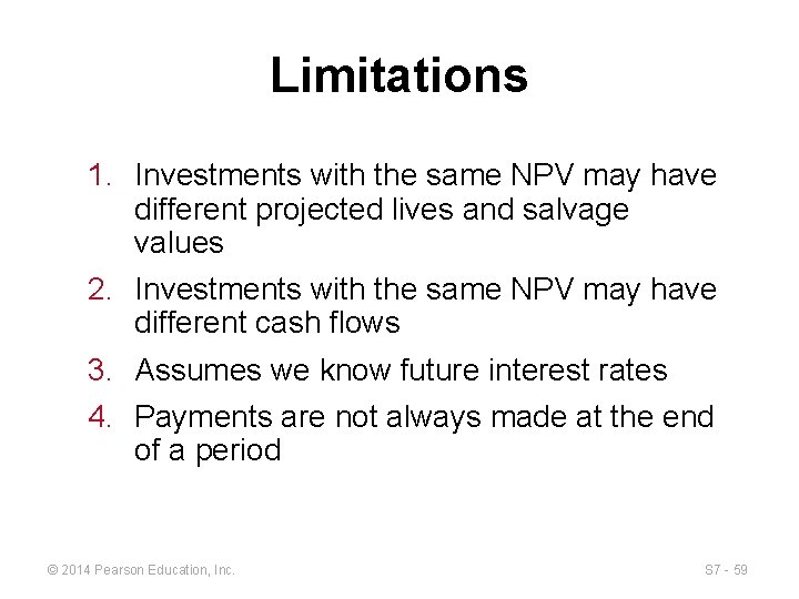
Limitations 1. Investments with the same NPV may have different projected lives and salvage values 2. Investments with the same NPV may have different cash flows 3. Assumes we know future interest rates 4. Payments are not always made at the end of a period © 2014 Pearson Education, Inc. S 7 - 59

All rights reserved. No part of this publication may be reproduced, stored in a retrieval system, or transmitted, in any form or by any means, electronic, mechanical, photocopying, recording, or otherwise, without the prior written permission of the publisher. Printed in the United States of America. © 2014 Pearson Education, Inc. S 7 - 60