Constraint management Constraint n n Something that limits

Constraint management

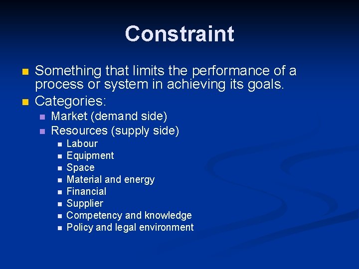
Constraint n n Something that limits the performance of a process or system in achieving its goals. Categories: n n Market (demand side) Resources (supply side) n n n n Labour Equipment Space Material and energy Financial Supplier Competency and knowledge Policy and legal environment

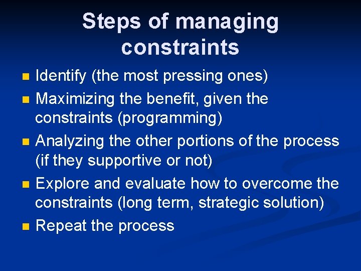
Steps of managing constraints n n n Identify (the most pressing ones) Maximizing the benefit, given the constraints (programming) Analyzing the other portions of the process (if they supportive or not) Explore and evaluate how to overcome the constraints (long term, strategic solution) Repeat the process

Linear programming

Linear programming… n n …is a quantitative management tool to obtain optimal solutions to problems that involve restrictions and limitations (called constrained optimization problems). …consists of a sequence of steps that lead to an optimal solution to linearconstrained problems, if an optimum exists.

Typical areas of problems n n n Determining optimal schedules Establishing locations Identifying optimal worker-job assignments Determining optimal diet plans Identifying optimal mix of products in a factory (!!!) etc.

Linear programming models n n …are mathematical representations of constrained optimization problems. BASIC CHARACTERISTICS: Components n Assumptions n

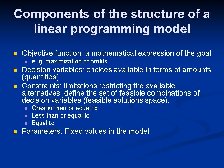
Components of the structure of a linear programming model n Objective function: a mathematical expression of the goal n n n Decision variables: choices available in terms of amounts (quantities) Constraints: limitations restricting the available alternatives; define the set of feasible combinations of decision variables (feasible solutions space). n n e. g. maximization of profits Greater than or equal to Less than or equal to Equal to Parameters. Fixed values in the model

Assumptions of the linear programming model n n Linearity: the impact of decision variables is linear in constraints and the objective functions Divisibility: noninteger values are acceptable Certainty: values of parameters are known and constant Nonnegativity: negative values of decision variables are not accepted

Model formulation n n 1. 2. 3. The procesess of assembling information about a problem into a model. This way the problem became solved mathematically. Identifying decision variables (e. g. quantity of a product) Identifying constraints Solve the problem.

Graphical linear programming 1. 2. 3. 4. 5. Set up the objective function and the constraints into mathematical format. Plot the constraints. Identify the feasible solution space. Plot the objective function. Determine the optimum solution. 1. 2. Sliding the line of the objective function away from the origin to the farthes/closest point of the feasible solution space. Enumeration approach.

Corporate system-matrix 1. ) Resource-product matrix Describes the connections between the company’s resources and products as linear and deterministic relations via coefficients of resource utilization and resource capacities. 2. ) Environmental matrix (or market-matrix): Describes the minimum that we must, and maximum that we can sell on the market from each product. It also describes the conditions.

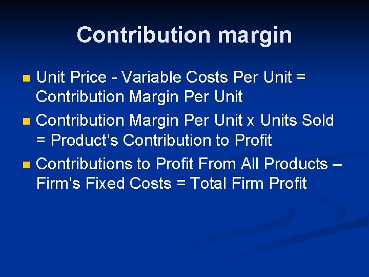
Contribution margin n Unit Price - Variable Costs Per Unit = Contribution Margin Per Unit x Units Sold = Product’s Contribution to Profit Contributions to Profit From All Products – Firm’s Fixed Costs = Total Firm Profit

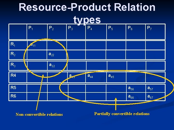
Resource-Product Relation types P 1 P 6 P 7 R 5 a 56 a 57 R 6 a 67 R 1 P 2 P 3 P 4 P 5 a 43 a 44 a 45 a 11 R 2 a 22 R 3 a 32 R 4 Non-convertible relations Partially convertible relations

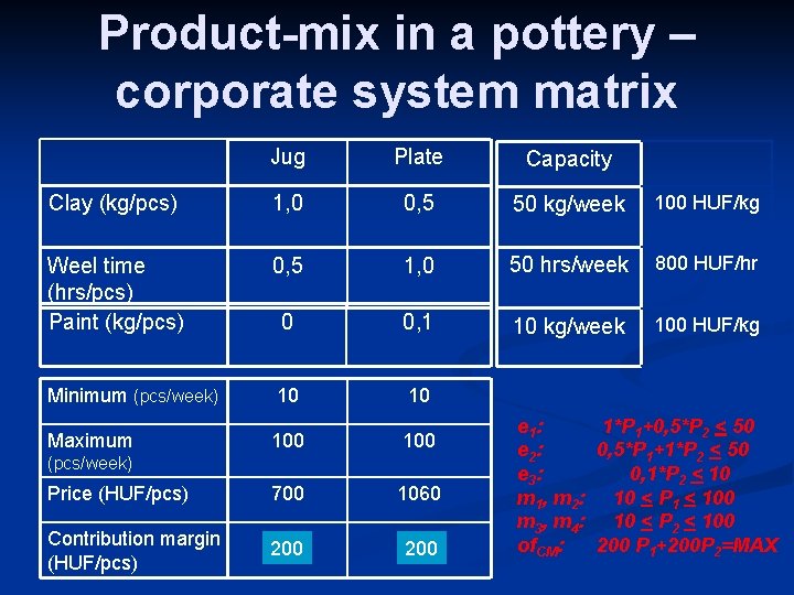
Product-mix in a pottery – corporate system matrix Jug Plate Capacity Clay (kg/pcs) 1, 0 0, 5 50 kg/week 100 HUF/kg Weel time (hrs/pcs) Paint (kg/pcs) 0, 5 1, 0 50 hrs/week 800 HUF/hr 0 0, 1 10 kg/week 100 HUF/kg Minimum (pcs/week) 10 10 Maximum 100 Price (HUF/pcs) 700 1060 Contribution margin (HUF/pcs) 200 (pcs/week) e 1 : 1*P 1+0, 5*P 2 < 50 e 2 : 0, 5*P 1+1*P 2 < 50 e 3 : 0, 1*P 2 < 10 m 1, m 2: 10 < P 1 < 100 m 3, m 4: 10 < P 2 < 100 of. CM: 200 P 1+200 P 2=MAX

Objective function n refers to choosing the best element from some set of available alternatives. X*P 1 + Y*P 2 = max weights (depends on what we want to maximize: price, contribution margin) variables (amount of produced goods)

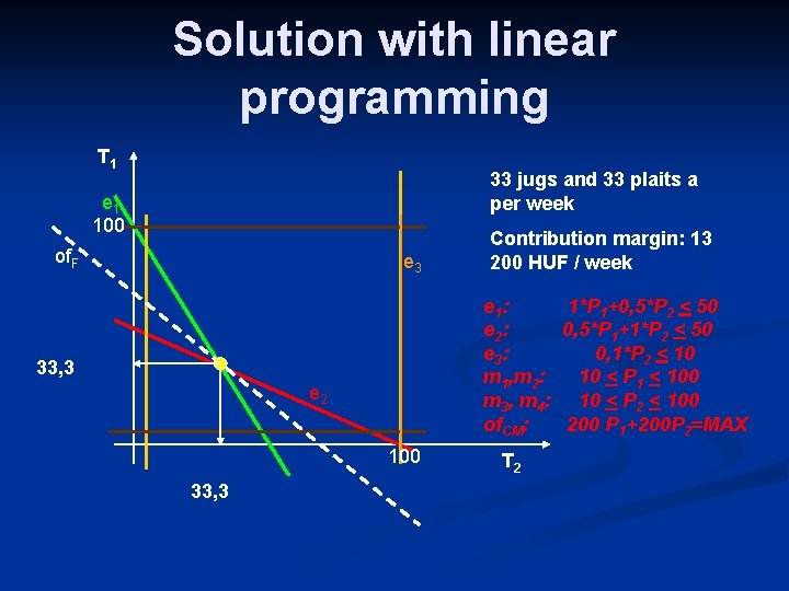
Solution with linear programming T 1 33 jugs and 33 plaits a per week e 1 100 of. F e 3 e 1 : 1*P 1+0, 5*P 2 < 50 e 2 : 0, 5*P 1+1*P 2 < 50 e 3 : 0, 1*P 2 < 10 m 1, m 2: 10 < P 1 < 100 m 3, m 4: 10 < P 2 < 100 of. CM: 200 P 1+200 P 2=MAX 33, 3 e 2 100 33, 3 Contribution margin: 13 200 HUF / week T 2

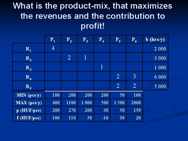
What is the product-mix, that maximizes the revenues and the contribution to profit! P 1 P 2 P 3 P 4 P 5 P 6 R 1 4 2 000 R 2 2 1 2 2 3 000 MIN (pcs/y) 100 200 200 50 100 MAX (pcs/y) 400 1100 1 000 500 1 500 2000 p (HUF/pcs) 200 270 200 30 50 150 f (HUF/pcs) 100 110 50 -10 30 20 R 3 R 4 R 5 b (hrs/y) 1 000 6 000 5 000

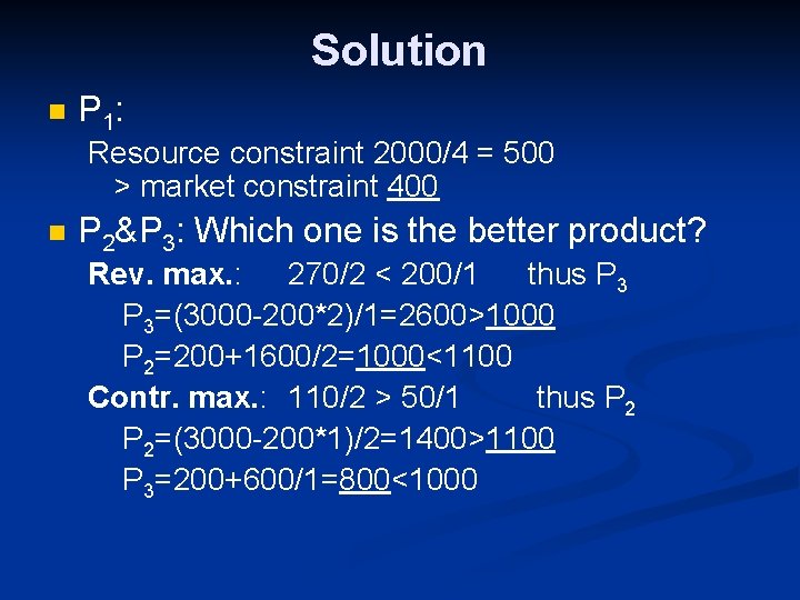
Solution n P 1: Resource constraint 2000/4 = 500 > market constraint 400 n P 2&P 3: Which one is the better product? Rev. max. : 270/2 < 200/1 thus P 3=(3000 -200*2)/1=2600>1000 P 2=200+1600/2=1000<1100 Contr. max. : 110/2 > 50/1 thus P 2=(3000 -200*1)/2=1400>1100 P 3=200+600/1=800<1000

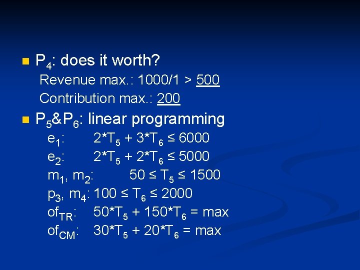
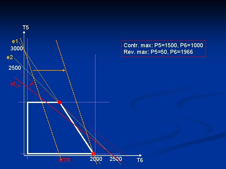
n P 4: does it worth? Revenue max. : 1000/1 > 500 Contribution max. : 200 n P 5&P 6: linear programming e 1: 2*T 5 + 3*T 6 ≤ 6000 e 2: 2*T 5 + 2*T 6 ≤ 5000 m 1 , m 2 : 50 ≤ T 5 ≤ 1500 p 3, m 4: 100 ≤ T 6 ≤ 2000 of. TR: 50*T 5 + 150*T 6 = max of. CM: 30*T 5 + 20*T 6 = max

T 5 e 1 3000 Contr. max: P 5=1500, P 6=1000 Rev. max: P 5=50, P 6=1966 e 2 2500 of. CM of. TR 2000 2500 T 6

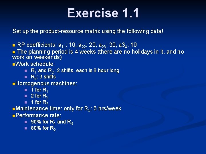
Exercise 1. 1 Set up the product-resource matrix using the following data! RP coefficients: a 11: 10, a 22: 20, a 23: 30, a 34: 10 n The planning period is 4 weeks (there are no holidays in it, and no work on weekends) n. Work schedule: n n n R 1 and R 2: 2 shifts, each is 8 hour long R 3: 3 shifts n. Homogenous n n n machines: 1 for R 1 2 for R 2 1 for R 3 n. Maintenance time: only for R 3: 5 hrs/week n. Performance rate: n n 90% for R 1 and R 3 80% for R 2

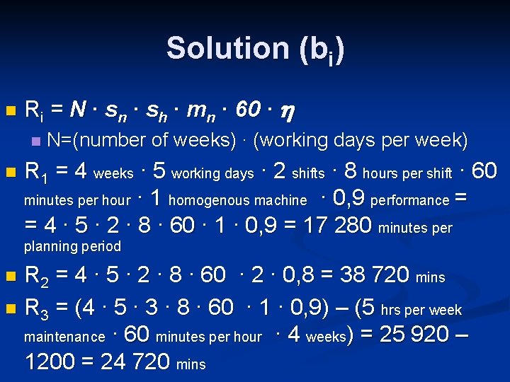
Solution (bi) n Ri = N ∙ sn ∙ sh ∙ mn ∙ 60 ∙ n n N=(number of weeks) ∙ (working days per week) R 1 = 4 weeks ∙ 5 working days ∙ 2 shifts ∙ 8 hours per shift ∙ 60 minutes per hour ∙ 1 homogenous machine ∙ 0, 9 performance = = 4 ∙ 5 ∙ 2 ∙ 8 ∙ 60 ∙ 1 ∙ 0, 9 = 17 280 minutes per planning period R 2 = 4 ∙ 5 ∙ 2 ∙ 8 ∙ 60 ∙ 2 ∙ 0, 8 = 38 720 mins n R 3 = (4 ∙ 5 ∙ 3 ∙ 8 ∙ 60 ∙ 1 ∙ 0, 9) – (5 hrs per week maintenance ∙ 60 minutes per hour ∙ 4 weeks) = 25 920 – 1200 = 24 720 mins n

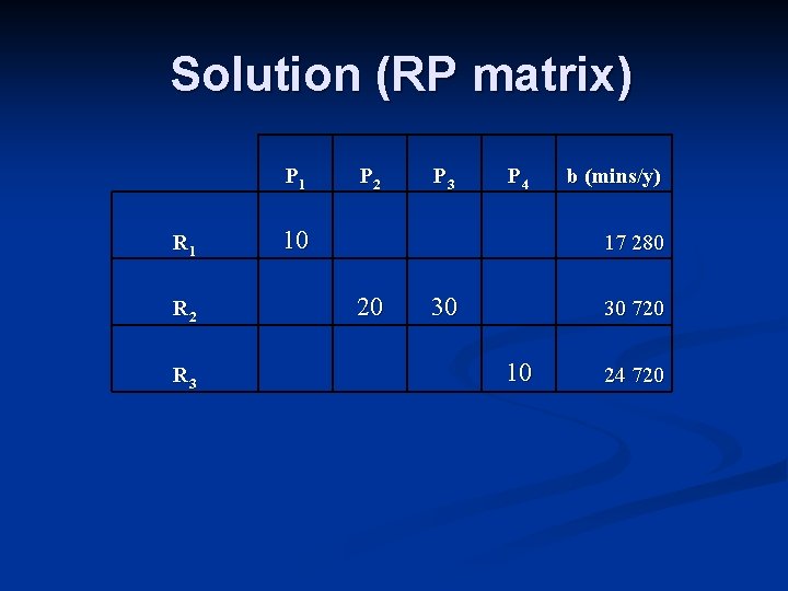
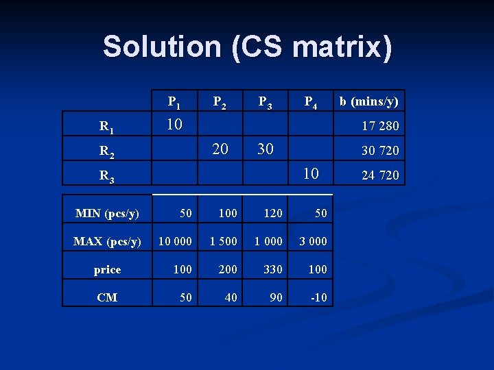
Solution (RP matrix) P 1 R 1 10 R 2 R 3 P 2 P 3 P 4 b (mins/y) 17 280 20 30 30 720 10 24 720

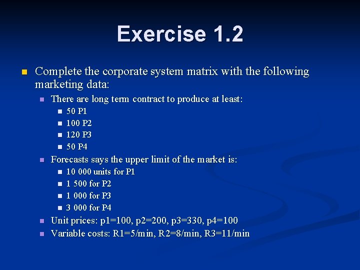
Exercise 1. 2 n Complete the corporate system matrix with the following marketing data: n There are long term contract to produce at least: n n n Forecasts says the upper limit of the market is: n n n 50 P 1 100 P 2 120 P 3 50 P 4 10 000 units for P 1 1 500 for P 2 1 000 for P 3 3 000 for P 4 Unit prices: p 1=100, p 2=200, p 3=330, p 4=100 Variable costs: R 1=5/min, R 2=8/min, R 3=11/min

Solution (CS matrix) P 1 R 1 10 P 2 P 4 b (mins/y) 17 280 20 R 2 P 3 30 30 720 10 R 3 MIN (pcs/y) 50 100 120 50 MAX (pcs/y) 10 000 1 500 1 000 3 000 price 100 200 330 100 CM 50 40 90 -10 24 720

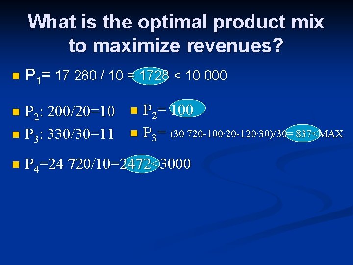
What is the optimal product mix to maximize revenues? n P 1= 17 280 / 10 = 1728 < 10 000 P 2: 200/20=10 n P 3: 330/30=11 n n P 2= 100 n P 3= (30 720 -100∙ 20 -120∙ 30)/30= 837<MAX n P 4=24 720/10=2472<3000

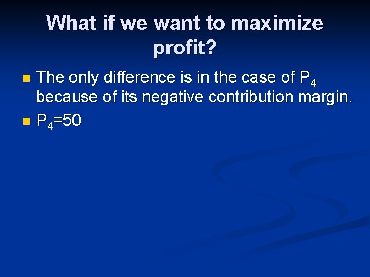
What if we want to maximize profit? The only difference is in the case of P 4 because of its negative contribution margin. n P 4=50 n

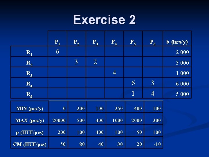
Exercise 2 P 1 P 2 P 3 P 4 P 5 P 6 b (hrs/y) R 1 6 3 2 000 4 6 1 3 4 1 000 R 2 R 3 R 4 R 5 MIN (pcs/y) 0 200 100 250 400 100 MAX (pcs/y) 20000 500 400 1000 200 p (HUF/pcs) 200 100 400 100 50 100 CM (HUF/pcs) 50 80 40 30 20 -10 3 000 6 000 5 000

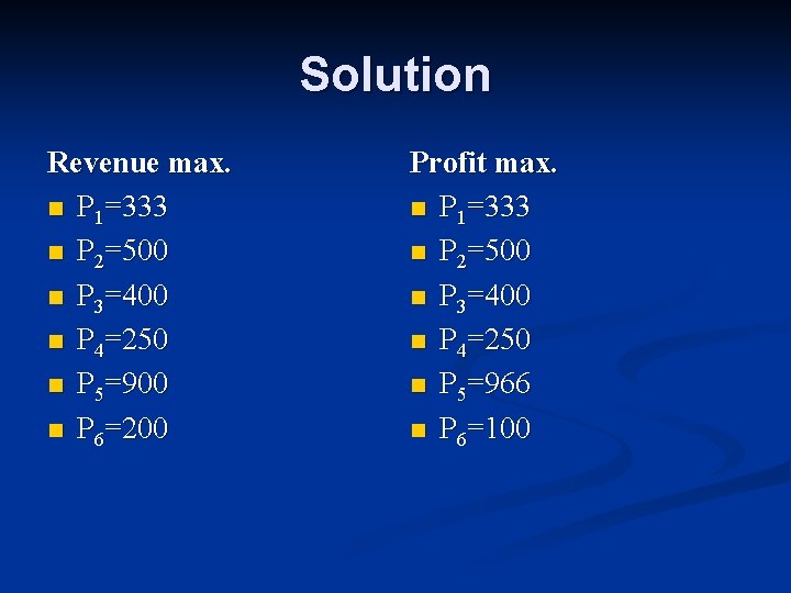
Solution Revenue max. n P 1=333 n P 2=500 n P 3=400 n P 4=250 n P 5=900 n P 6=200 Profit max. n P 1=333 n P 2=500 n P 3=400 n P 4=250 n P 5=966 n P 6=100