Computational Social Choice Lirong Xia IJCAI13 Tutorial Aug

Computational Social Choice Lirong Xia IJCAI-13 Tutorial Aug 4, 2013

A shameless advertisement… • About RPI – The first technological institutes in English-speaking countries – Graduate school rankings in US • 47 th Computer Science • 28 th Computer Engineering • 17 th Applied Math • I am generally interested in both theory and application of economics and computation. – Hiring highly motivated Ph. D. students – If interested, please send me an email (xial@cs. rpi. edu) 1

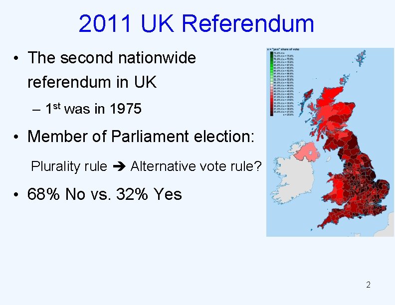
2011 UK Referendum • The second nationwide referendum in UK – 1 st was in 1975 • Member of Parliament election: Plurality rule Alternative vote rule? • 68% No vs. 32% Yes 2

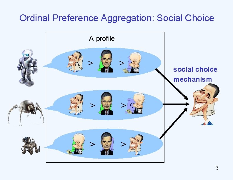
Ordinal Preference Aggregation: Social Choice A profile Alice Bob Carol A > B > C > social choice mechanism A A 3

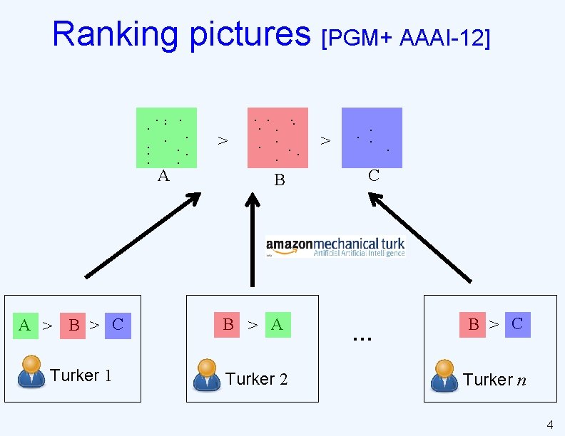
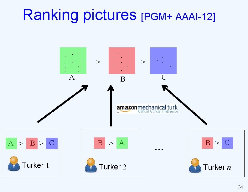
Ranking pictures [PGM+ AAAI-12]. . . . A A > B > C Turker 1 . . . > . . . B B > A Turker 2 > . . C … B > C Turker n 4

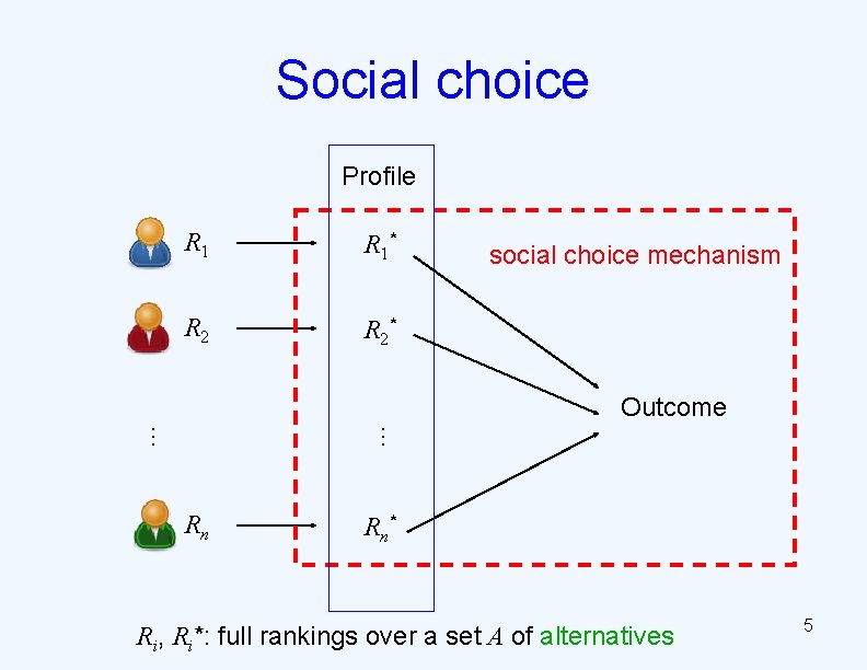
Social choice Profile R 1* R 2* social choice mechanism Outcome … … Rn R n* Ri, Ri*: full rankings over a set A of alternatives 5

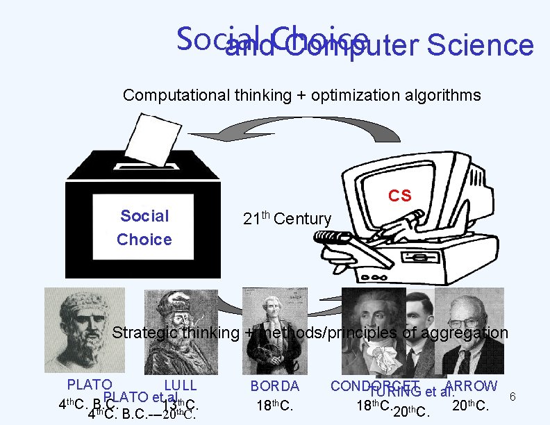
Social Choice and Computer Science Computational thinking + optimization algorithms CS Social Choice 21 th Century Strategic thinking + methods/principles of aggregation PLATO LULL PLATO et al. th 4 th. C. B. C. 13 C. 4 th. C. B. C. ---20 th. C. BORDA 18 th. C. CONDORCET ARROW TURING et al. 18 th. C. 20 th. C. 6

Applications: real world • People/agents often have conflicting preferences, yet they have to make a joint decision 7

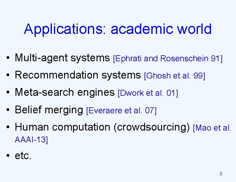
Applications: academic world • Multi-agent systems [Ephrati and Rosenschein 91] • Recommendation systems [Ghosh et al. 99] • Meta-search engines [Dwork et al. 01] • Belief merging [Everaere et al. 07] • Human computation (crowdsourcing) [Mao et al. AAAI-13] • etc. 8

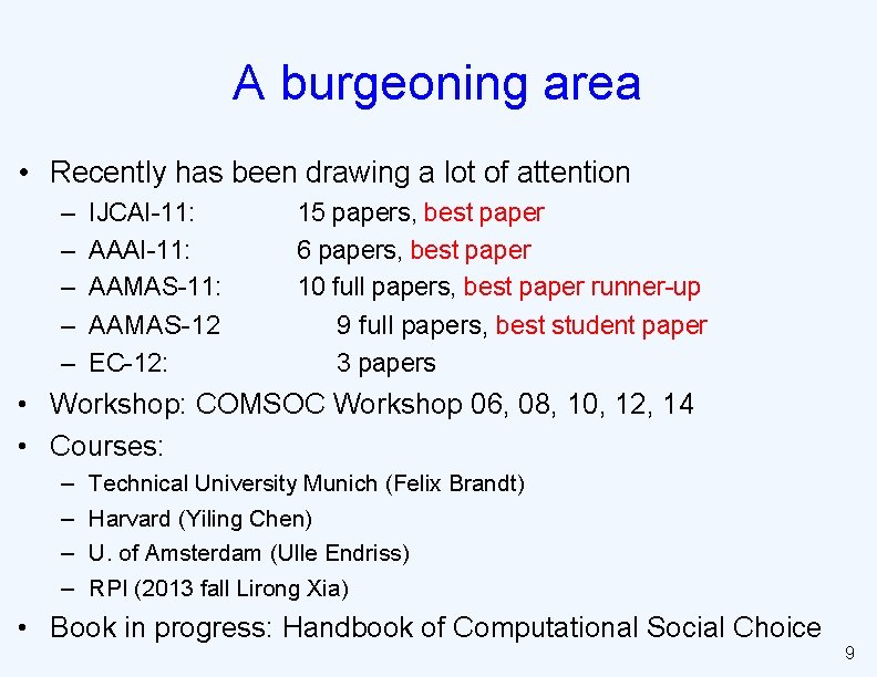
A burgeoning area • Recently has been drawing a lot of attention – – – IJCAI-11: 15 papers, best paper AAAI-11: 6 papers, best paper AAMAS-11: 10 full papers, best paper runner-up AAMAS-12 EC-12: 9 full papers, best student paper 3 papers • Workshop: COMSOC Workshop 06, 08, 10, 12, 14 • Courses: – – Technical University Munich (Felix Brandt) Harvard (Yiling Chen) U. of Amsterdam (Ulle Endriss) RPI (2013 fall Lirong Xia) • Book in progress: Handbook of Computational Social Choice 9

Flavor of this tutorial • High-level objectives for – design – evaluation – logic flow among research topics “Give a man a fish and you feed him for a day. Teach a man to fish and you feed him for a lifetime. ” -----Chinese proverb • Plus some concrete results 10

How to design a good social What is being “good”? choice mechanism? 11

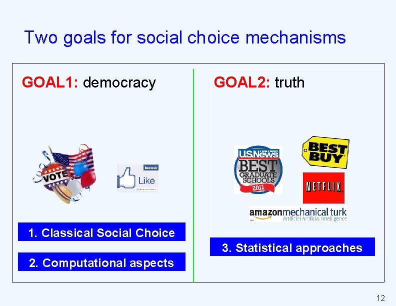
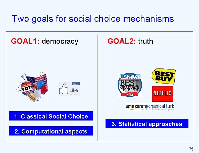
Two goals for social choice mechanisms GOAL 1: democracy GOAL 2: truth 1. Classical Social Choice 3. Statistical approaches 2. Computational aspects 12

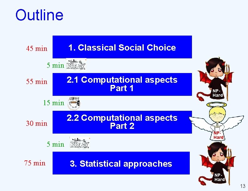
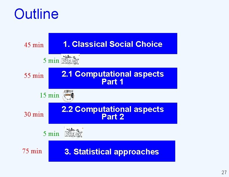
Outline 45 min 1. Classical Social Choice 5 min 55 min 2. 1 Computational aspects Part 1 NPHard 15 min 30 min 2. 2 Computational aspects Part 2 NPHard 5 min 75 min 3. Statistical approaches NPHard 13

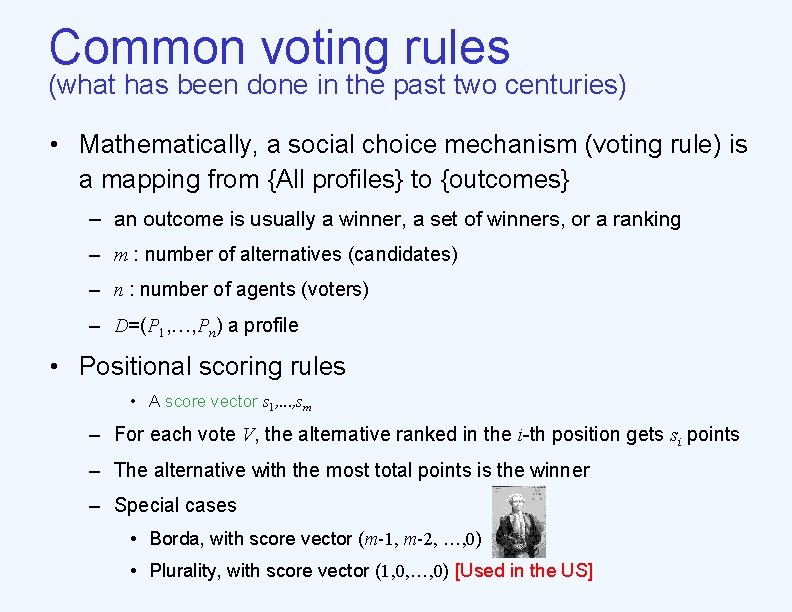
Common voting rules (what has been done in the past two centuries) • Mathematically, a social choice mechanism (voting rule) is a mapping from {All profiles} to {outcomes} – an outcome is usually a winner, a set of winners, or a ranking – m : number of alternatives (candidates) – n : number of agents (voters) – D=(P 1, …, Pn) a profile • Positional scoring rules • A score vector s 1, . . . , sm – For each vote V, the alternative ranked in the i-th position gets si points – The alternative with the most total points is the winner – Special cases • Borda, with score vector (m-1, m-2, …, 0) • Plurality, with score vector (1, 0, …, 0) [Used in the US]

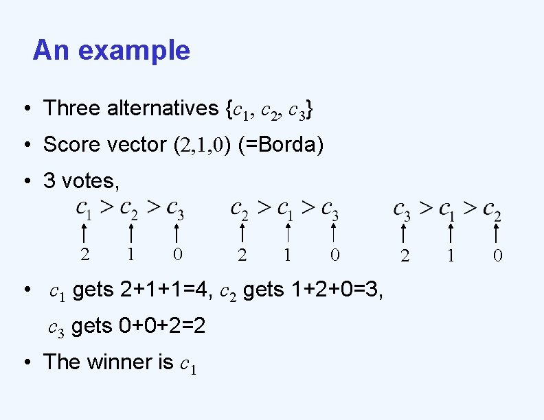
An example • Three alternatives {c 1, c 2, c 3} • Score vector (2, 1, 0) (=Borda) • 3 votes, 2 1 0 • c 1 gets 2+1+1=4, c 2 gets 1+2+0=3, c 3 gets 0+0+2=2 • The winner is c 1 2 1 0

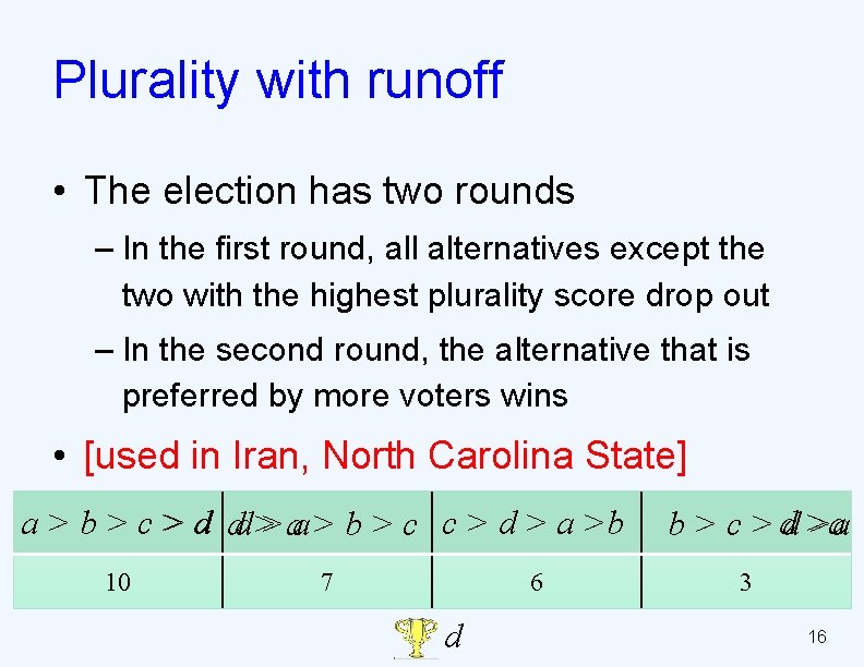
Plurality with runoff • The election has two rounds – In the first round, all alternatives except the two with the highest plurality score drop out – In the second round, the alternative that is preferred by more voters wins • [used in Iran, North Carolina State] a > b > c > d dd >> aa > b > c c > d > a >b 10 7 6 d b > c > dd >a >a 3 16

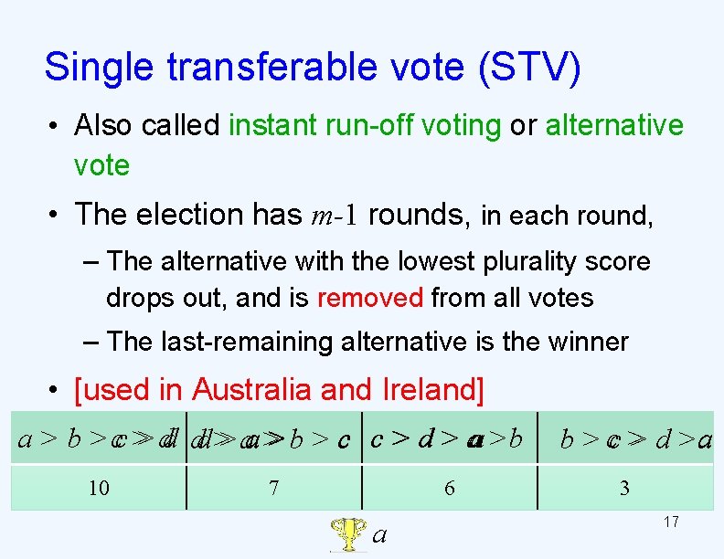
Single transferable vote (STV) • Also called instant run-off voting or alternative vote • The election has m-1 rounds, in each round, – The alternative with the lowest plurality score drops out, and is removed from all votes – The last-remaining alternative is the winner • [used in Australia and Ireland] a > b > cc > > dd dd >> aa >> b > c c > d > aa >b 10 7 6 a a b > c > d >a 3 17

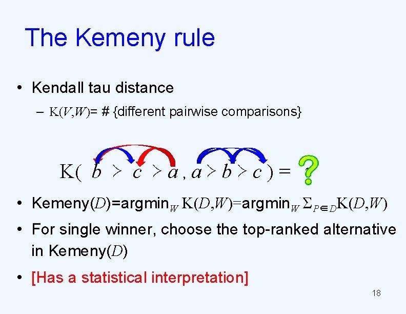
The Kemeny rule • Kendall tau distance – K(V, W)= # {different pairwise comparisons} K( b ≻ c ≻ a , a ≻ b ≻ c ) = 21 • Kemeny(D)=argmin. W K(D, W)=argmin. W ΣP∈DK(D, W) • For single winner, choose the top-ranked alternative in Kemeny(D) • [Has a statistical interpretation] 18

…and many others • Approval, Baldwin, Black, Bucklin, Coombs, Copeland, Dodgson, maximin, Nanson, Range voting, Schulze, Slater, ranked pairs, etc… 19

• Q: How to evaluate rules in terms of achieving democracy? • A: Axiomatic approach 20

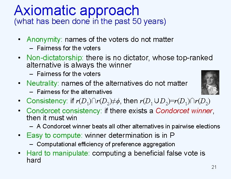
Axiomatic approach (what has been done in the past 50 years) • Anonymity: names of the voters do not matter – Fairness for the voters • Non-dictatorship: there is no dictator, whose top-ranked alternative is always the winner – Fairness for the voters • Neutrality: names of the alternatives do not matter – Fairness for the alternatives • Consistency: if r(D 1)∩r(D 2)≠ϕ, then r(D 1∪D 2)=r(D 1)∩r(D 2) • Condorcet consistency: if there exists a Condorcet winner, then it must win – A Condorcet winner beats all other alternatives in pairwise elections • Easy to compute: winner determination is in P – Computational efficiency of preference aggregation • Hard to manipulate: computing a beneficial false vote is hard 21

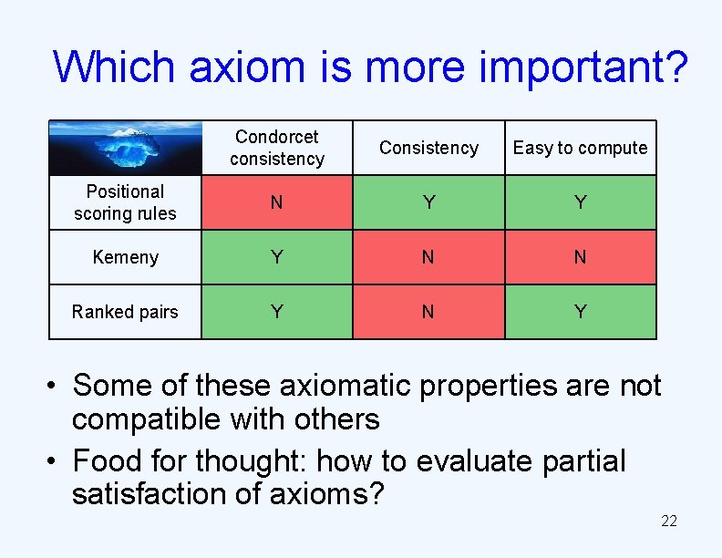
Which axiom is more important? Condorcet consistency Consistency Easy to compute Positional scoring rules N Y Y Kemeny Y N N Ranked pairs Y N Y • Some of these axiomatic properties are not compatible with others • Food for thought: how to evaluate partial satisfaction of axioms? 22

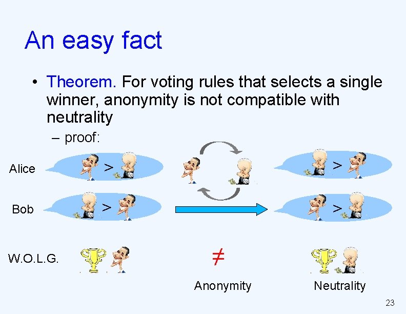
An easy fact • Theorem. For voting rules that selects a single winner, anonymity is not compatible with neutrality – proof: Alice > > Bob > > W. O. L. G. ≠ Anonymity Neutrality 23

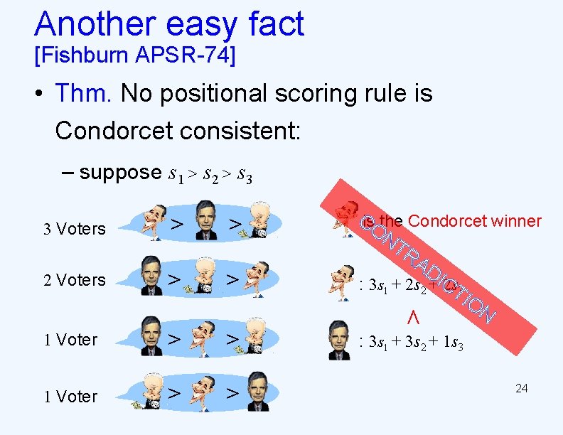
Another easy fact [Fishburn APSR-74] • Thm. No positional scoring rule is Condorcet consistent: – suppose s 1 > s 2 > s 3 > 2 Voters > > 1 Voter > > Cis the Condorcet winner ON TR AD : 3 s 1 + 2 s 2 +IC 2 s. T 3 IO N < 3 Voters > : 3 s 1 + 3 s 2 + 1 s 3 24

Not-So-Easy facts • Arrow’s impossibility theorem – Google it! • Gibbard-Satterthwaite theorem – Next section • Axiomatic characterization – Template: A voting rule satisfies axioms A 1, A 2 if it is rule X – If you believe in A 1 A 2 A 3 are the most desirable properties then X is optimal – (anonymity+neutrality+consistency+continuity) positional scoring rules [Young SIAMAM-75] – (neutrality+consistency+Condorcet consistency) Kemeny [Young&Levenglick SIAMAM-78] 25

Food for thought • Can we quantify a voting rule’s satisfiability of these axiomatic properties? – Tradeoffs between satisfiability of axioms – Use computational techniques to design new voting rules • use AI techniques to automatically prove or discover new impossibility theorems [Tang&Lin AIJ-09] 26

Outline 45 min 1. Classical Social Choice 5 min 55 min 2. 1 Computational aspects Part 1 15 min 30 min 2. 2 Computational aspects Part 2 5 min 75 min 3. Statistical approaches 27

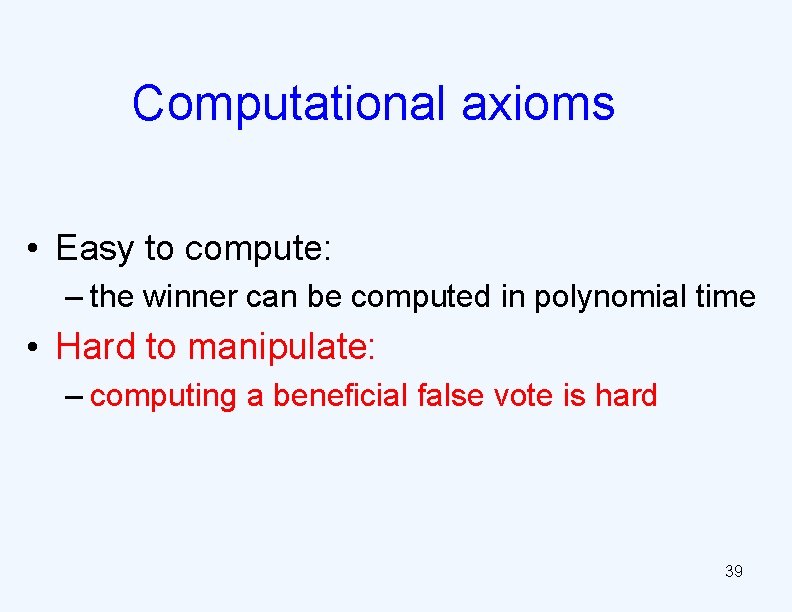
Computational axioms • Easy to compute: – the winner can be computed in polynomial time • Hard to manipulate: – computing a beneficial false vote is hard 28

Computational axioms • Easy to compute: – the winner can be computed in polynomial time • Hard to manipulate: – computing a beneficial false vote is hard 29

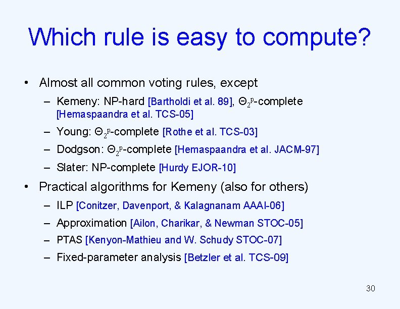
Which rule is easy to compute? • Almost all common voting rules, except – Kemeny: NP-hard [Bartholdi et al. 89], Θ 2 p-complete [Hemaspaandra et al. TCS-05] – Young: Θ 2 p-complete [Rothe et al. TCS-03] – Dodgson: Θ 2 p-complete [Hemaspaandra et al. JACM-97] – Slater: NP-complete [Hurdy EJOR-10] • Practical algorithms for Kemeny (also for others) – ILP [Conitzer, Davenport, & Kalagnanam AAAI-06] – Approximation [Ailon, Charikar, & Newman STOC-05] – PTAS [Kenyon-Mathieu and W. Schudy STOC-07] – Fixed-parameter analysis [Betzler et al. TCS-09] 30

Really easy to compute? • Easy to compute axiom: computing the winner takes polynomial time in the input size – input size: nmlog m • What if m is extremely large? 31

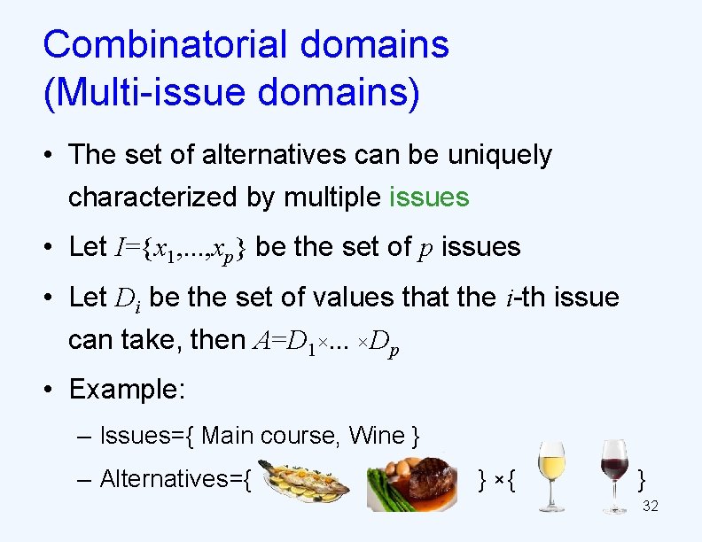
Combinatorial domains (Multi-issue domains) • The set of alternatives can be uniquely characterized by multiple issues • Let I={x 1, . . . , xp} be the set of p issues • Let Di be the set of values that the i-th issue can take, then A=D 1×. . . ×Dp • Example: – Issues={ Main course, Wine } – Alternatives={ } ×{ } 32

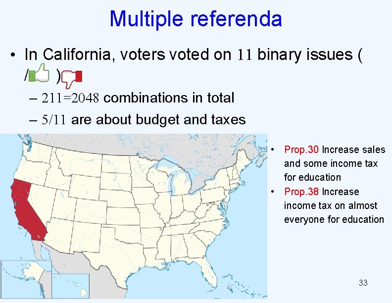
Multiple referenda • In California, voters voted on 11 binary issues ( / ) – 211=2048 combinations in total – 5/11 are about budget and taxes • Prop. 30 Increase sales and some income tax for education • Prop. 38 Increase income tax on almost everyone for education 33

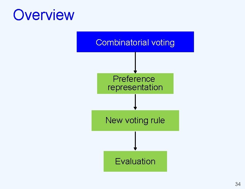
Overview Combinatorial voting Preference representation New voting rule Evaluation 34

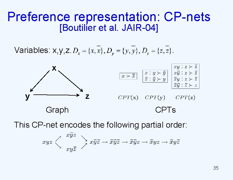
Preference representation: CP-nets [Boutilier et al. JAIR-04] Variables: x, y, z. x y z Graph CPTs This CP-net encodes the following partial order: 35

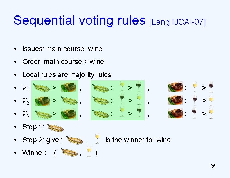
Sequential voting rules [Lang IJCAI-07] • Issues: main course, wine • Order: main course > wine • Local rules are majority rules • V 1: > , : > • V 2: > , : > • V 3: > , : > • Step 1: • Step 2: given , is the winner for wine • Winner: ( , ) 36

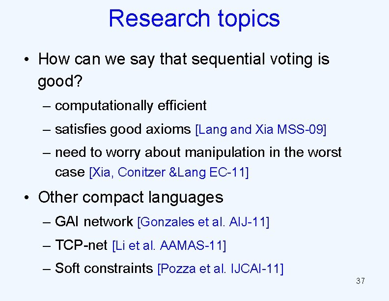
Research topics • How can we say that sequential voting is good? – computationally efficient – satisfies good axioms [Lang and Xia MSS-09] – need to worry about manipulation in the worst case [Xia, Conitzer &Lang EC-11] • Other compact languages – GAI network [Gonzales et al. AIJ-11] – TCP-net [Li et al. AAMAS-11] – Soft constraints [Pozza et al. IJCAI-11] 37

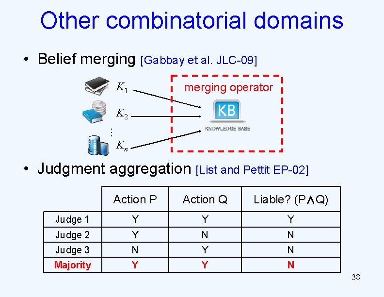
Other combinatorial domains • Belief merging [Gabbay et al. JLC-09] K 1 merging operator K 2 … Kn • Judgment aggregation [List and Pettit EP-02] Action P Action Q Liable? (P∧Q) Judge 1 Y Y Y Judge 2 Y N N Judge 3 N Y N Majority Y Y N 38

Computational axioms • Easy to compute: – the winner can be computed in polynomial time • Hard to manipulate: – computing a beneficial false vote is hard 39

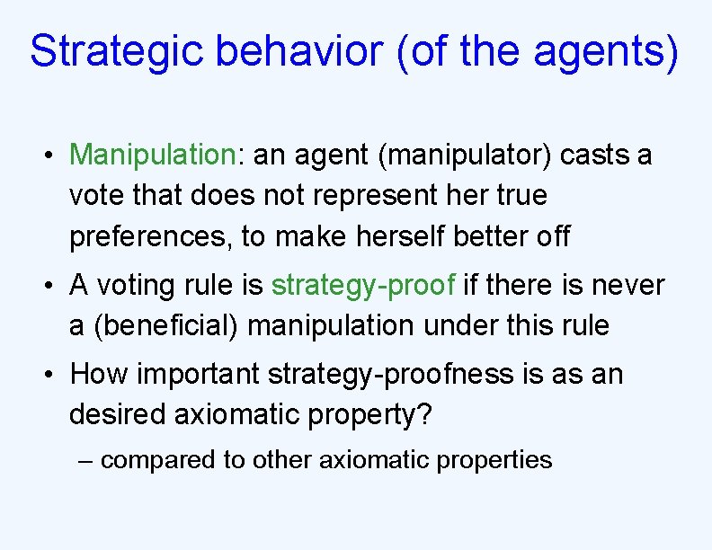
Strategic behavior (of the agents) • Manipulation: an agent (manipulator) casts a vote that does not represent her true preferences, to make herself better off • A voting rule is strategy-proof if there is never a (beneficial) manipulation under this rule • How important strategy-proofness is as an desired axiomatic property? – compared to other axiomatic properties

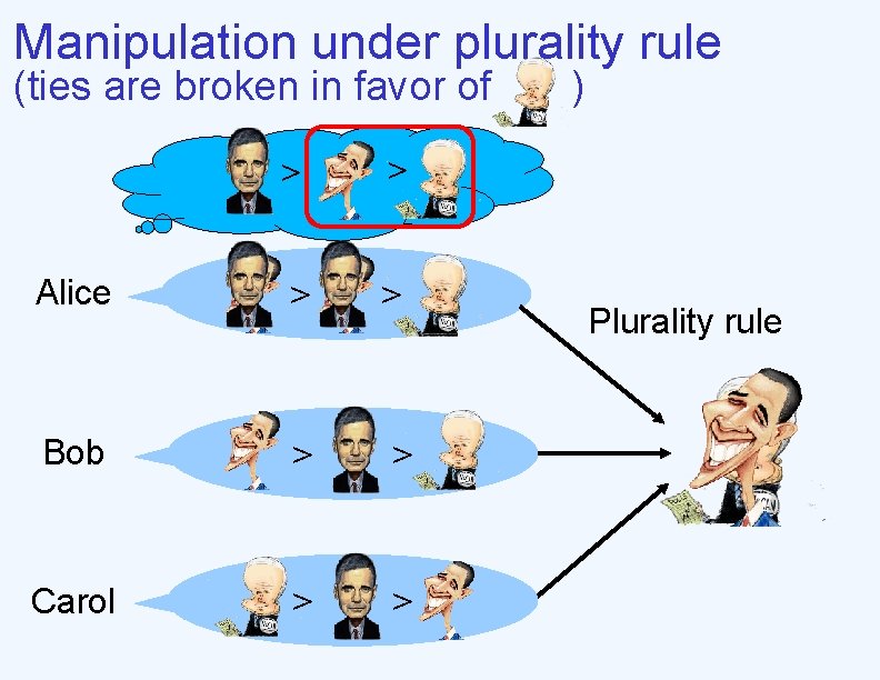
Manipulation under plurality rule (ties are broken in favor of ) > > Alice > > Bob > > Carol > > Plurality rule

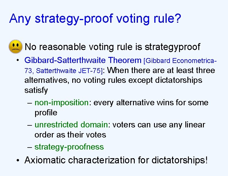
Any strategy-proof voting rule? • No reasonable voting rule is strategyproof • Gibbard-Satterthwaite Theorem [Gibbard Econometrica 73, Satterthwaite JET-75]: When there at least three alternatives, no voting rules except dictatorships satisfy – non-imposition: every alternative wins for some profile – unrestricted domain: voters can use any linear order as their votes – strategy-proofness • Axiomatic characterization for dictatorships!

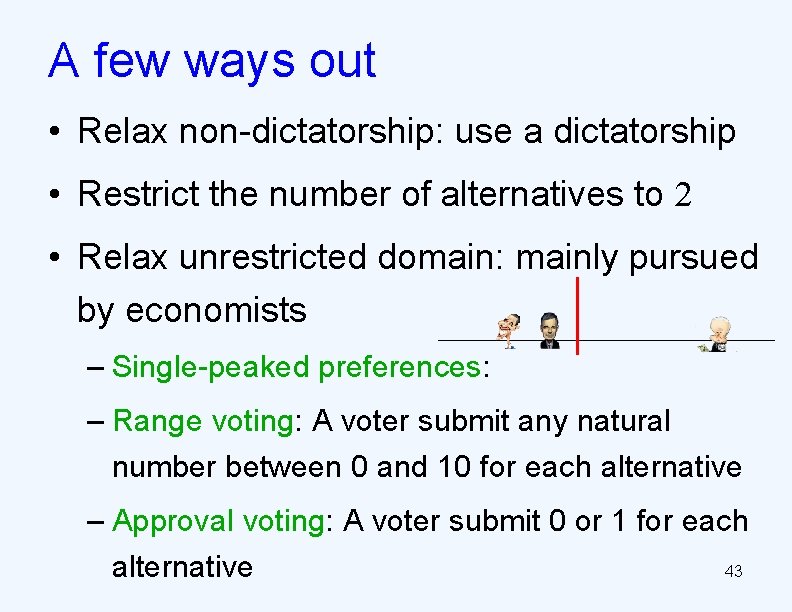
A few ways out • Relax non-dictatorship: use a dictatorship • Restrict the number of alternatives to 2 • Relax unrestricted domain: mainly pursued by economists – Single-peaked preferences: – Range voting: A voter submit any natural number between 0 and 10 for each alternative – Approval voting: A voter submit 0 or 1 for each 43 alternative

Computational thinking • Use a voting rule that is too complicated so that nobody can easily predict the winner – Dodgson – Kemeny – The randomized voting rule used in Venice Republic for more than 500 years [Walsh&Xia AAMAS-12] • We want a voting rule where – Winner determination is easy – Manipulation is hard 44

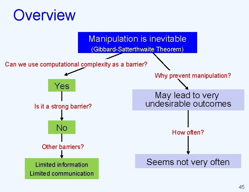
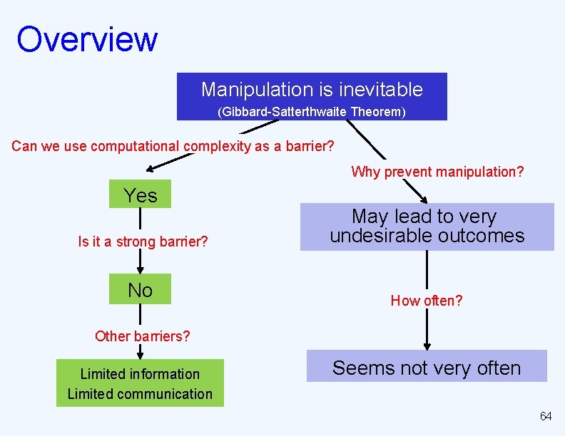
Overview Manipulation is inevitable (Gibbard-Satterthwaite Theorem) Can we use computational complexity as a barrier? Why prevent manipulation? Yes Is it a strong barrier? No May lead to very undesirable outcomes How often? Other barriers? Limited information Limited communication Seems not very often 45

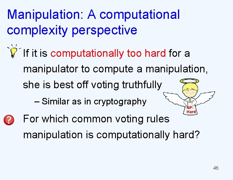
Manipulation: A computational complexity perspective If it is computationally too hard for a manipulator to compute a manipulation, she is best off voting truthfully – Similar as in cryptography NPHard For which common voting rules manipulation is computationally hard? 46

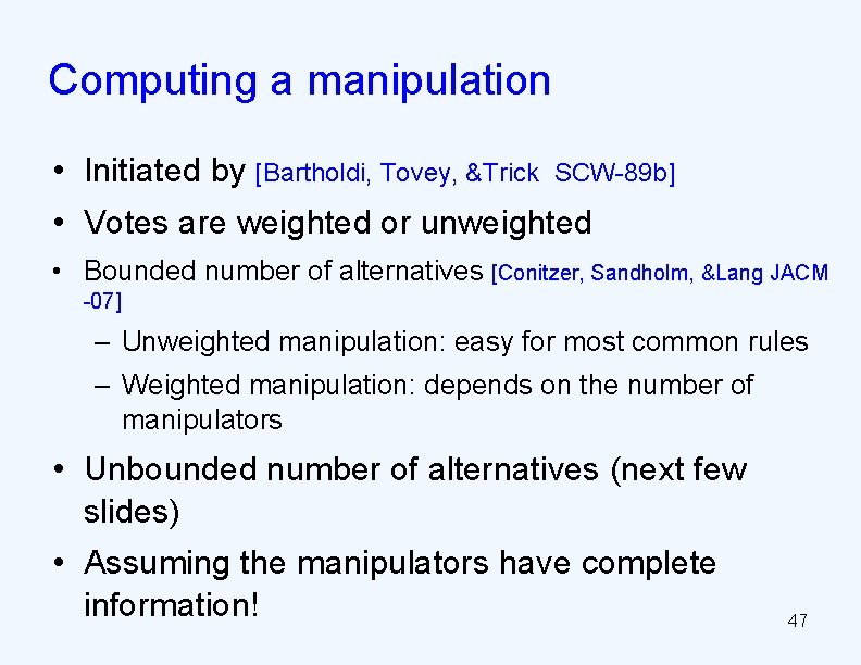
Computing a manipulation • Initiated by [Bartholdi, Tovey, &Trick SCW-89 b] • Votes are weighted or unweighted • Bounded number of alternatives [Conitzer, Sandholm, &Lang JACM -07] – Unweighted manipulation: easy for most common rules – Weighted manipulation: depends on the number of manipulators • Unbounded number of alternatives (next few slides) • Assuming the manipulators have complete information! 47

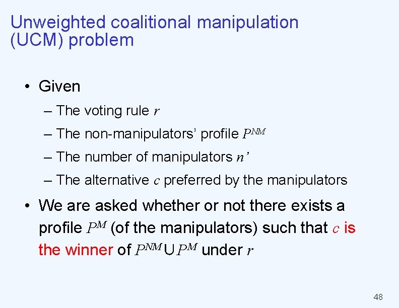
Unweighted coalitional manipulation (UCM) problem • Given – The voting rule r – The non-manipulators’ profile PNM – The number of manipulators n’ – The alternative c preferred by the manipulators • We are asked whether or not there exists a profile PM (of the manipulators) such that c is the winner of PNM∪PM under r 48

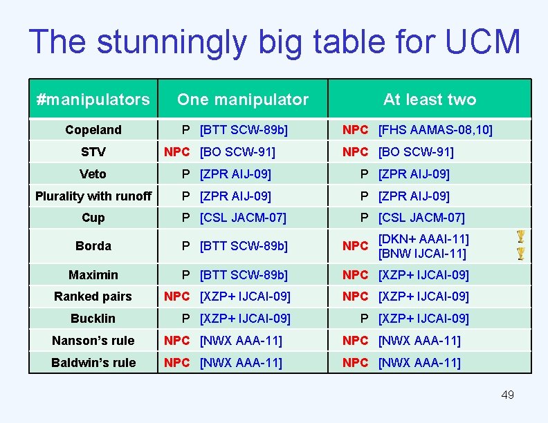
The stunningly big table for UCM #manipulators Copeland STV One manipulator P [BTT SCW-89 b] NPC [BO SCW-91] At least two NPC [FHS AAMAS-08, 10] NPC [BO SCW-91] Veto P [ZPR AIJ-09] Plurality with runoff P [ZPR AIJ-09] Cup P [CSL JACM-07] Borda P [BTT SCW-89 b] NPC Maximin P [BTT SCW-89 b] NPC [XZP+ IJCAI-09] P [XZP+ IJCAI-09] Ranked pairs Bucklin [DKN+ AAAI-11] [BNW IJCAI-11] Nanson’s rule NPC [NWX AAA-11] Baldwin’s rule NPC [NWX AAA-11] 49

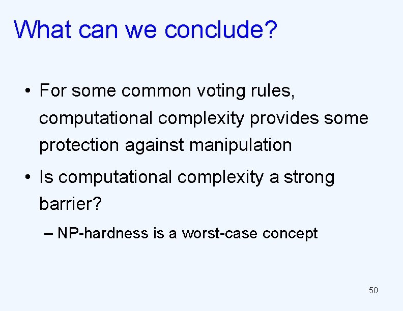
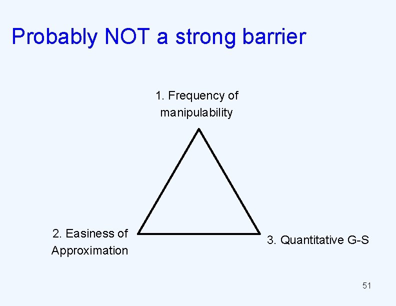
What can we conclude? • For some common voting rules, computational complexity provides some protection against manipulation • Is computational complexity a strong barrier? – NP-hardness is a worst-case concept 50

Probably NOT a strong barrier 1. Frequency of manipulability 2. Easiness of Approximation 3. Quantitative G-S 51

A first angle: frequency of manipulability • Non-manipulators’ votes are drawn i. i. d. – E. g. i. i. d. uniformly over all linear orders (the impartial culture assumption) • How often can the manipulators make c win? – Specific voting rules [Peleg T&D-79, Baharad&Neeman RED-02, Slinko T&D-02, Slinko MSS-04, Procaccia and Rosenschein AAMAS-07] 52

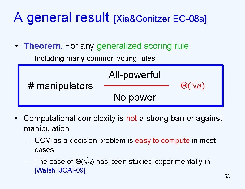
A general result [Xia&Conitzer EC-08 a] • Theorem. For any generalized scoring rule – Including many common voting rules All-powerful # manipulators Θ(√n) No power • Computational complexity is not a strong barrier against manipulation – UCM as a decision problem is easy to compute in most cases – The case of Θ(√n) has been studied experimentally in [Walsh IJCAI-09] 53

A second angle: approximation • Unweighted coalitional optimization (UCO): compute the smallest number of manipulators that can make c win – A greedy algorithm has additive error no more than 1 for Borda [Zuckerman, Procaccia, &Rosenschein AIJ-09] 54

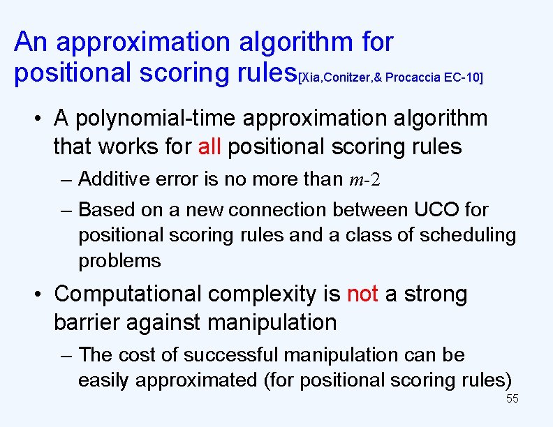
An approximation algorithm for positional scoring rules[Xia, Conitzer, & Procaccia EC-10] • A polynomial-time approximation algorithm that works for all positional scoring rules – Additive error is no more than m-2 – Based on a new connection between UCO for positional scoring rules and a class of scheduling problems • Computational complexity is not a strong barrier against manipulation – The cost of successful manipulation can be easily approximated (for positional scoring rules) 55

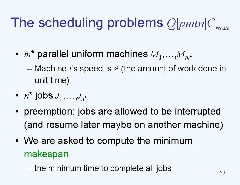
The scheduling problems Q|pmtn|Cmax • m* parallel uniform machines M 1, …, Mm* – Machine i’s speed is si (the amount of work done in unit time) • n* jobs J 1, …, Jn* • preemption: jobs are allowed to be interrupted (and resume later maybe on another machine) • We are asked to compute the minimum makespan – the minimum time to complete all jobs 56

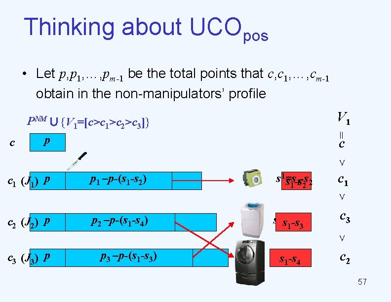
Thinking about UCOpos • Let p, p 1, …, pm-1 be the total points that c, c 1, …, cm-1 obtain in the non-manipulators’ profile = c V 1 PNM ∪{V 1=[c>c 1>c 2>c 3]} p c ∨ c 1 (J 1) p p 1 –p-(s p 11 -s-p 2) s 1=s s 1 -s 22 c 1 ∨ c 2 (J 2) p p 2 –p-(s p 21 p-s 2 4 -p ) s 2=s s 1 -s 33 c 3 ∨ c 3 (J 3) p p 3 –p-(s p 3 p 1 -s 3 -p 3) s 3 s=s 1 -s 14 -s 4 c 2 57

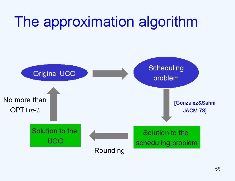
The approximation algorithm Scheduling problem Original UCO No more than OPT+m-2 [Gonzalez&Sahni JACM 78] Solution to the UCO Rounding Solution to the scheduling problem 58

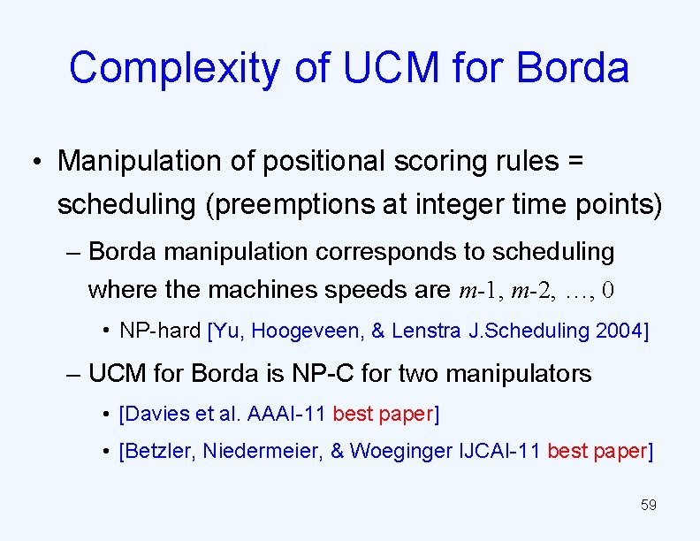
Complexity of UCM for Borda • Manipulation of positional scoring rules = scheduling (preemptions at integer time points) – Borda manipulation corresponds to scheduling where the machines speeds are m-1, m-2, …, 0 • NP-hard [Yu, Hoogeveen, & Lenstra J. Scheduling 2004] – UCM for Borda is NP-C for two manipulators • [Davies et al. AAAI-11 best paper] • [Betzler, Niedermeier, & Woeginger IJCAI-11 best paper] 59

A third angle: quantitative G-S • G-S theorem: for any reasonable voting rule there exists a manipulation • Quantitative G-S: for any voting rule that is “far away” from dictatorships, the number of manipulable situations is non-negligible – First work: 3 alternatives, neutral rule [Friedgut, Kalai, &Nisan FOCS-08] – Extensions: [Dobzinski&Procaccia WINE-08, Xia&Conitzer EC-08 b, Isaksson, Kindler, &Mossel FOCS-10] – Finally proved: [Mossel&Racz STOC-12] 60

Next steps • The first attempt seems to fail • Can we obtain positive results for a restricted setting? – The manipulators has complete information about the non-manipulators’ votes – The manipulators can perfectly discuss their strategies 61

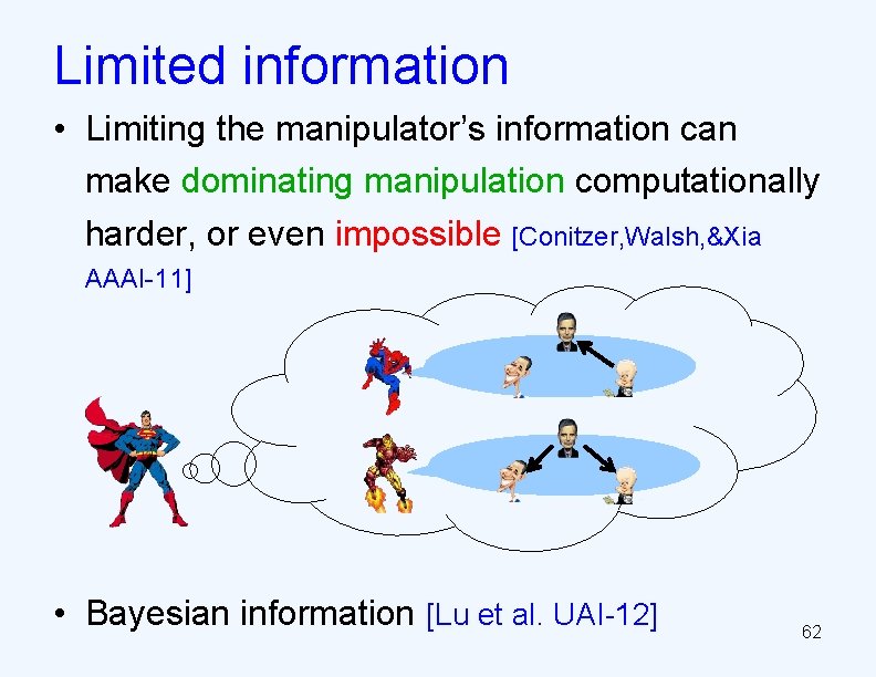
Limited information • Limiting the manipulator’s information can make dominating manipulation computationally harder, or even impossible [Conitzer, Walsh, &Xia AAAI-11] • Bayesian information [Lu et al. UAI-12] 62

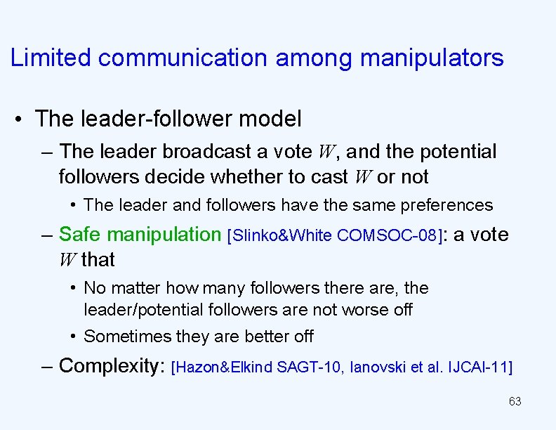
Limited communication among manipulators • The leader-follower model – The leader broadcast a vote W, and the potential followers decide whether to cast W or not • The leader and followers have the same preferences – Safe manipulation [Slinko&White COMSOC-08]: a vote W that • No matter how many followers there are, the leader/potential followers are not worse off • Sometimes they are better off – Complexity: [Hazon&Elkind SAGT-10, Ianovski et al. IJCAI-11] 63

Overview Manipulation is inevitable (Gibbard-Satterthwaite Theorem) Can we use computational complexity as a barrier? Why prevent manipulation? Yes Is it a strong barrier? No May lead to very undesirable outcomes How often? Other barriers? Limited information Limited communication Seems not very often 64

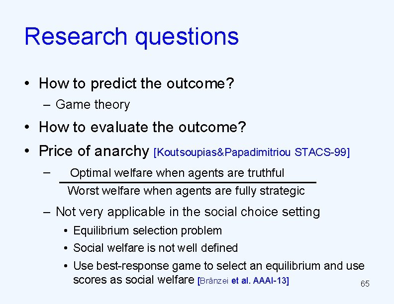
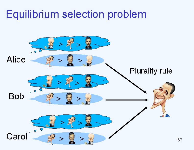
Research questions • How to predict the outcome? – Game theory • How to evaluate the outcome? • Price of anarchy [Koutsoupias&Papadimitriou STACS-99] – Optimal welfare when agents are truthful Worst welfare when agents are fully strategic – Not very applicable in the social choice setting • Equilibrium selection problem • Social welfare is not well defined • Use best-response game to select an equilibrium and use scores as social welfare [Brânzei et al. AAAI-13] 65

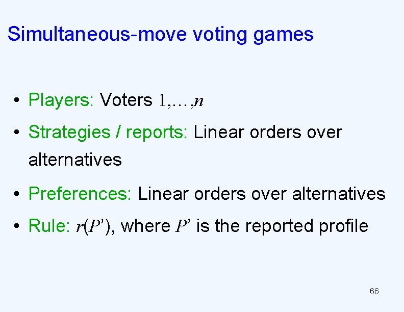
Simultaneous-move voting games • Players: Voters 1, …, n • Strategies / reports: Linear orders over alternatives • Preferences: Linear orders over alternatives • Rule: r(P’), where P’ is the reported profile 66

Equilibrium selection problem Alice > > Plurality rule Bob Carol > > > > 67

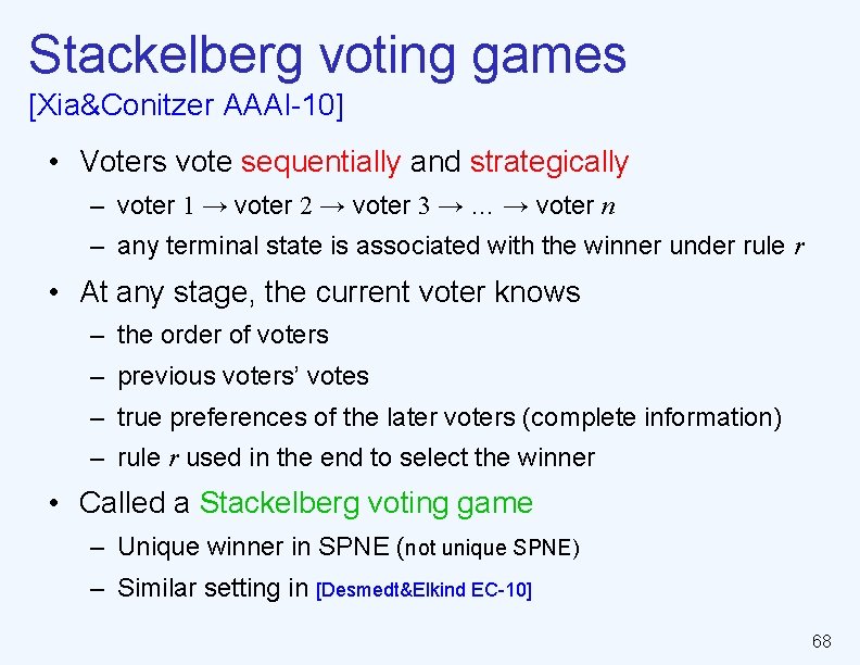
Stackelberg voting games [Xia&Conitzer AAAI-10] • Voters vote sequentially and strategically – voter 1 → voter 2 → voter 3 → … → voter n – any terminal state is associated with the winner under rule r • At any stage, the current voter knows – the order of voters – previous voters’ votes – true preferences of the later voters (complete information) – rule r used in the end to select the winner • Called a Stackelberg voting game – Unique winner in SPNE (not unique SPNE) – Similar setting in [Desmedt&Elkind EC-10] 68

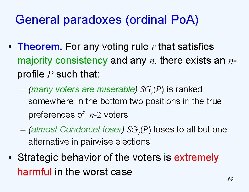
General paradoxes (ordinal Po. A) • Theorem. For any voting rule r that satisfies majority consistency and any n, there exists an nprofile P such that: – (many voters are miserable) SGr(P) is ranked somewhere in the bottom two positions in the true preferences of n-2 voters – (almost Condorcet loser) SGr(P) loses to all but one alternative in pairwise elections • Strategic behavior of the voters is extremely harmful in the worst case 69

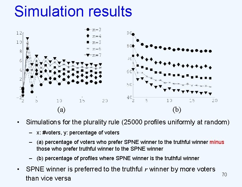
Simulation results (a) (b) • Simulations for the plurality rule (25000 profiles uniformly at random) – x: #voters, y: percentage of voters – (a) percentage of voters who prefer SPNE winner to the truthful winner minus those who prefer truthful winner to the SPNE winner – (b) percentage of profiles where SPNE winner is the truthful winner • SPNE winner is preferred to the truthful r winner by more voters than vice versa 70

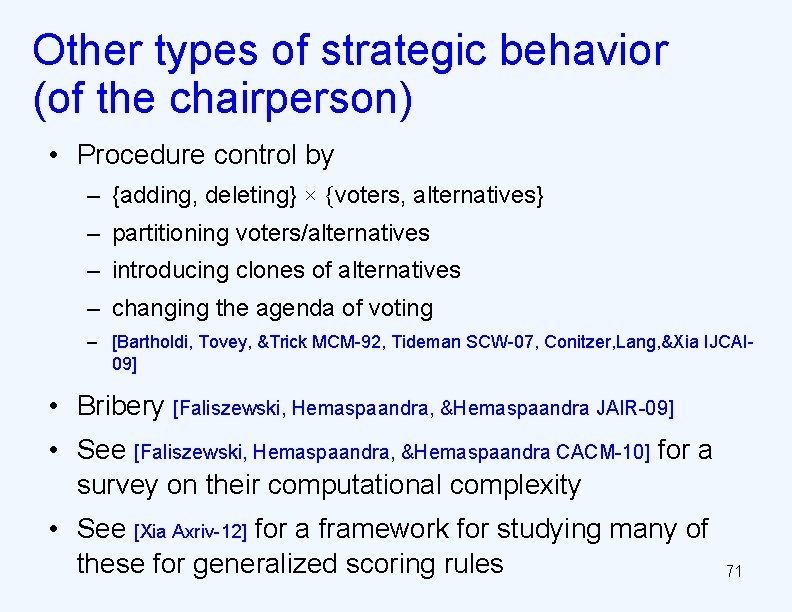
Other types of strategic behavior (of the chairperson) • Procedure control by – {adding, deleting} × {voters, alternatives} – partitioning voters/alternatives – introducing clones of alternatives – changing the agenda of voting – [Bartholdi, Tovey, &Trick MCM-92, Tideman SCW-07, Conitzer, Lang, &Xia IJCAI 09] • Bribery [Faliszewski, Hemaspaandra, &Hemaspaandra JAIR-09] • See [Faliszewski, Hemaspaandra, &Hemaspaandra CACM-10] for a survey on their computational complexity • See [Xia Axriv-12] for a framework for studying many of these for generalized scoring rules 71

Food for thought • The problem is still very open! – Shown to be connected to integer factorization [Hemaspaandra, & Menton STACS-13] • What is the role of computational complexity in analyzing human/self-interested agents’ behavior? – Explore information/communication assumptions – In general, why do we want to prevent strategic behavior? • Practical ways to protect elections 72

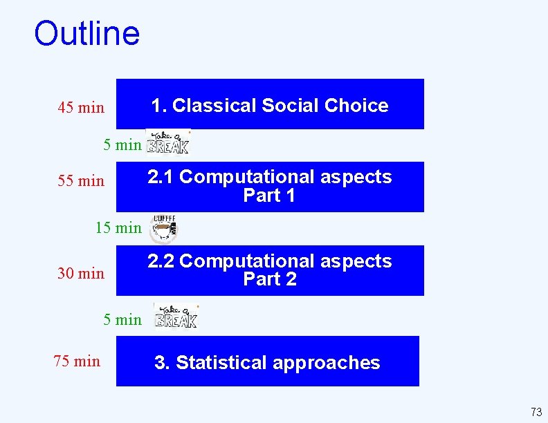
Outline 45 min 1. Classical Social Choice 5 min 55 min 2. 1 Computational aspects Part 1 15 min 30 min 2. 2 Computational aspects Part 2 5 min 75 min 3. Statistical approaches 73

Ranking pictures [PGM+ AAAI-12]. . . . A A > B > C Turker 1 . . . > . . . B B > A Turker 2 > . . C … B > C Turker n 74

Two goals for social choice mechanisms GOAL 1: democracy GOAL 2: truth 1. Classical Social Choice 3. Statistical approaches 2. Computational aspects 75

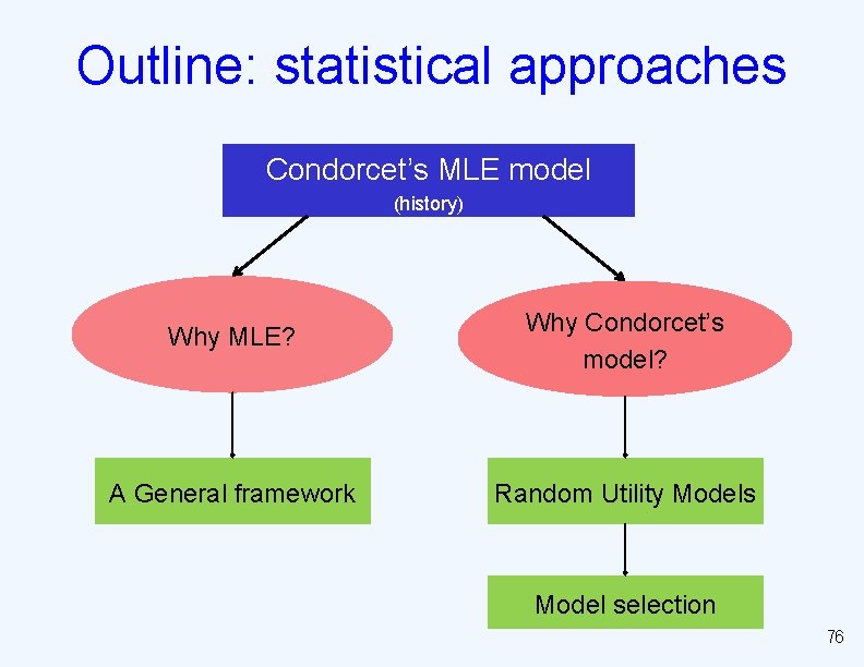
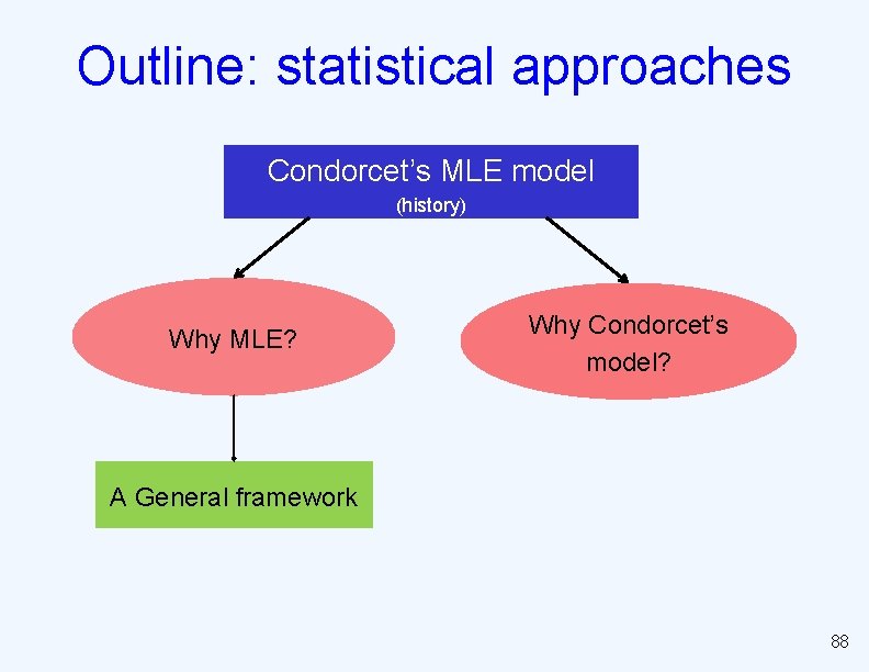
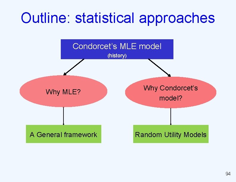
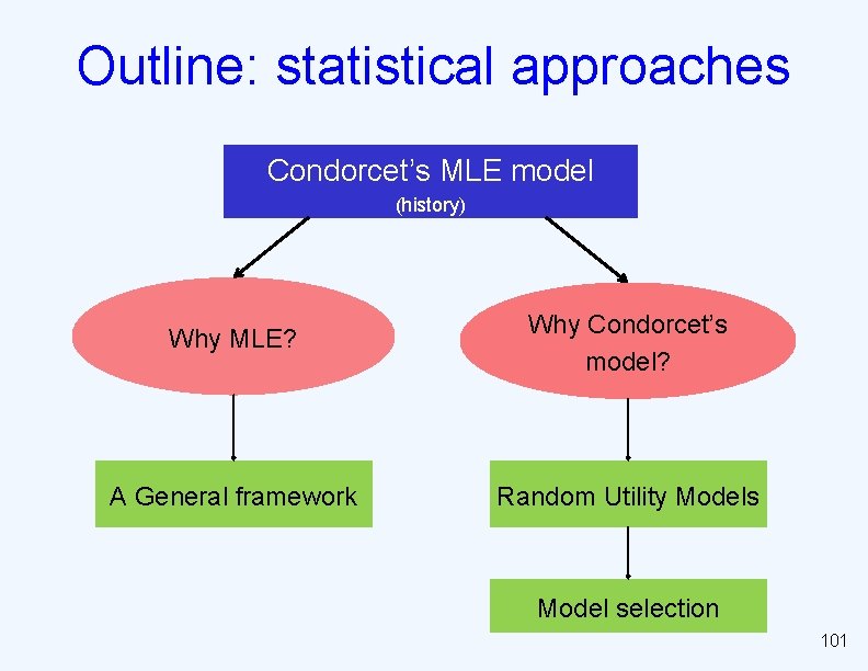
Outline: statistical approaches Condorcet’s MLE model (history) Why MLE? Why Condorcet’s model? A General framework Random Utility Models Model selection 76

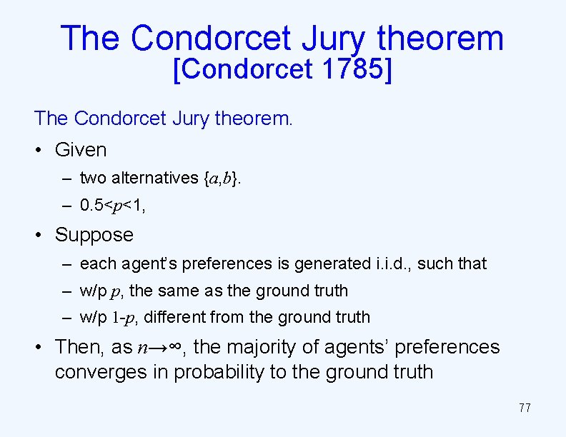
The Condorcet Jury theorem [Condorcet 1785] The Condorcet Jury theorem. • Given – two alternatives {a, b}. – 0. 5<p<1, • Suppose – each agent’s preferences is generated i. i. d. , such that – w/p p, the same as the ground truth – w/p 1 -p, different from the ground truth • Then, as n→∞, the majority of agents’ preferences converges in probability to the ground truth 77

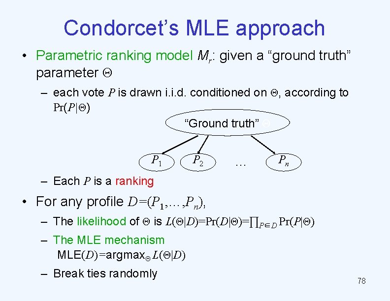
Condorcet’s MLE approach • Parametric ranking model Mr: given a “ground truth” parameter Θ – each vote P is drawn i. i. d. conditioned on Θ, according to Pr(P|Θ) “Ground truth” Θ P 1 P 2 … Pn – Each P is a ranking • For any profile D=(P 1, …, Pn), – The likelihood of Θ is L(Θ|D)=Pr(D|Θ)=∏P∈D Pr(P|Θ) – The MLE mechanism MLE(D)=argmaxΘ L(Θ|D) – Break ties randomly 78

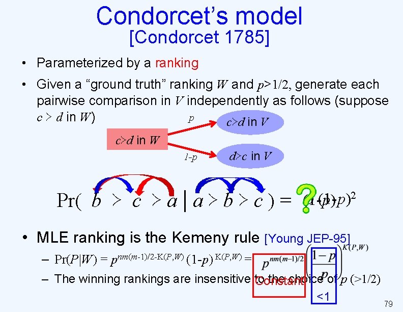
Condorcet’s model [Condorcet 1785] • Parameterized by a ranking • Given a “ground truth” ranking W and p>1/2, generate each pairwise comparison in V independently as follows (suppose p c ≻ d in W) c≻d in V c≻d in W 1 -p d≻c in V Pr( b ≻ c ≻ a | a ≻ b ≻ c ) = p (1 -p)2 (1 -p) • MLE ranking is the Kemeny rule [Young JEP-95] – Pr(P|W) = pnm(m-1)/2 -K(P, W) (1 -p) K(P, W) = – The winning rankings are insensitive to the choice of p (>1/2) Constant <1 79

Recent studies on Condorcet’s model • Learning [Lu and Boutilier ICML-11] • Approximation by common voting rules [Caragiannis, Procaccia & Shah EC-13] 80

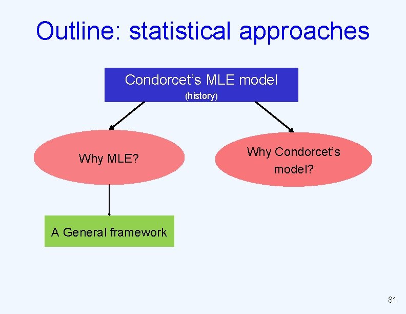
Outline: statistical approaches Condorcet’s MLE model (history) Why MLE? Why Condorcet’s model? A General framework 81

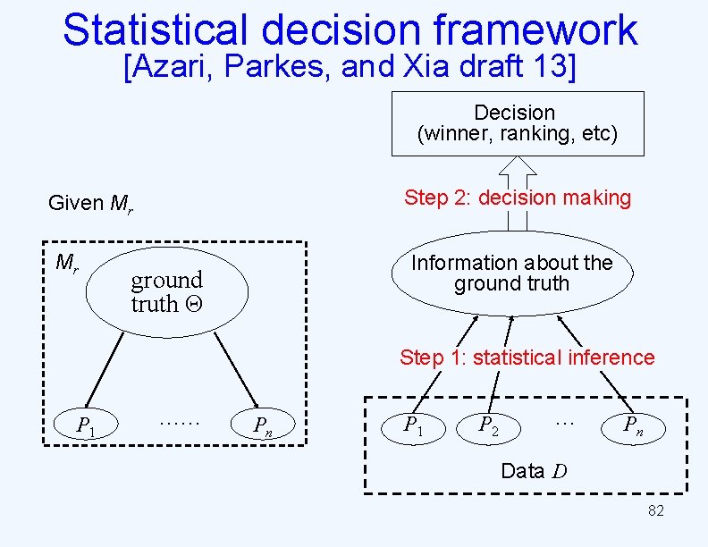
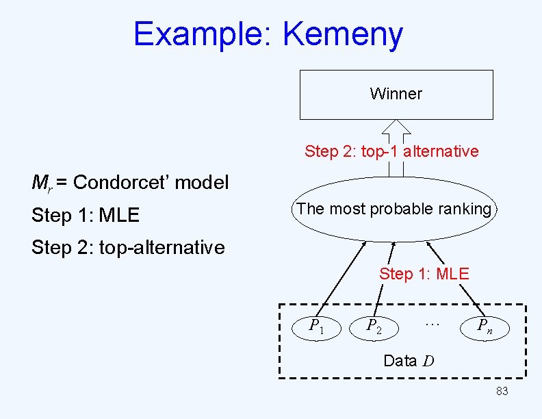
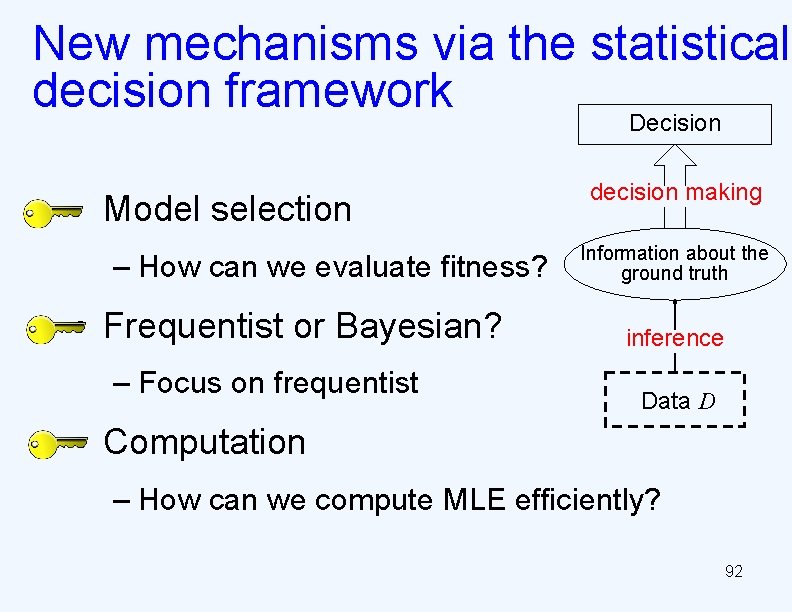
Statistical decision framework [Azari, Parkes, and Xia draft 13] Decision (winner, ranking, etc) Step 2: decision making Given Mr Mr Information about the ground truth Θ Step 1: statistical inference P 1 …… Pn P 1 P 2 … Pn Data D 82

Example: Kemeny Winner Step 2: top-1 alternative Mr = Condorcet’ model Step 1: MLE The most probable ranking Step 2: top-alternative Step 1: MLE P 1 P 2 … Pn Data D 83

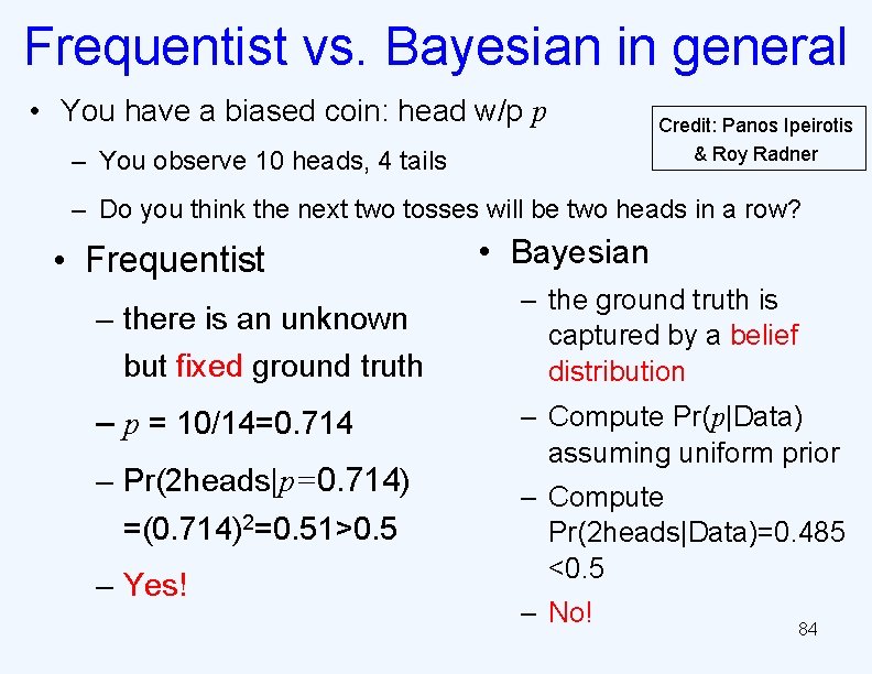
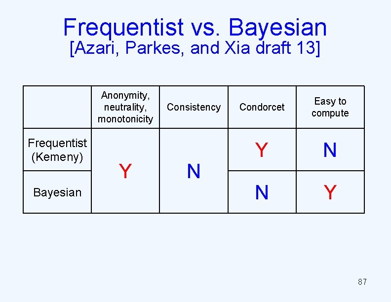
Frequentist vs. Bayesian in general • You have a biased coin: head w/p p – You observe 10 heads, 4 tails Credit: Panos Ipeirotis & Roy Radner – Do you think the next two tosses will be two heads in a row? • Frequentist • Bayesian – there is an unknown but fixed ground truth – the ground truth is captured by a belief distribution – p = 10/14=0. 714 – Compute Pr(p|Data) assuming uniform prior – Pr(2 heads|p=0. 714) =(0. 714)2=0. 51>0. 5 – Yes! – Compute Pr(2 heads|Data)=0. 485 <0. 5 – No! 84

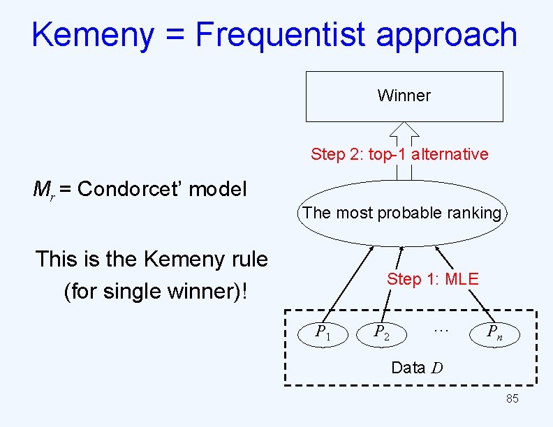
Kemeny = Frequentist approach Winner Step 2: top-1 alternative Mr = Condorcet’ model The most probable ranking This is the Kemeny rule (for single winner)! Step 1: MLE P 1 P 2 … Pn Data D 85

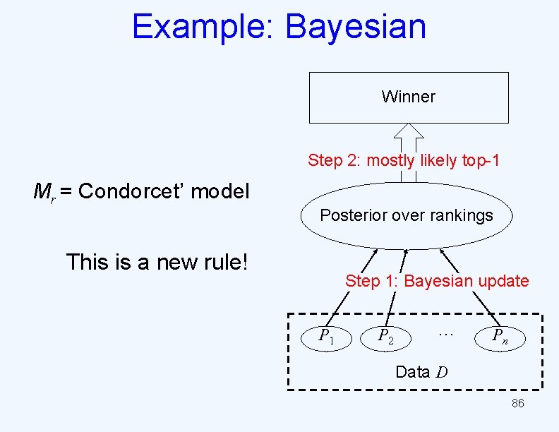
Example: Bayesian Winner Step 2: mostly likely top-1 Mr = Condorcet’ model Posterior over rankings This is a new rule! Step 1: Bayesian update P 1 P 2 … Pn Data D 86

Frequentist vs. Bayesian [Azari, Parkes, and Xia draft 13] Anonymity, neutrality, monotonicity Frequentist (Kemeny) Bayesian Y Consistency N Condorcet Easy to compute Y N N Y 87

Outline: statistical approaches Condorcet’s MLE model (history) Why MLE? Why Condorcet’s model? A General framework 88

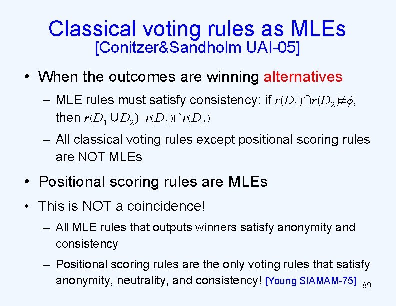
Classical voting rules as MLEs [Conitzer&Sandholm UAI-05] • When the outcomes are winning alternatives – MLE rules must satisfy consistency: if r(D 1)∩r(D 2)≠ϕ, then r(D 1∪D 2)=r(D 1)∩r(D 2) – All classical voting rules except positional scoring rules are NOT MLEs • Positional scoring rules are MLEs • This is NOT a coincidence! – All MLE rules that outputs winners satisfy anonymity and consistency – Positional scoring rules are the only voting rules that satisfy anonymity, neutrality, and consistency! [Young SIAMAM-75] 89

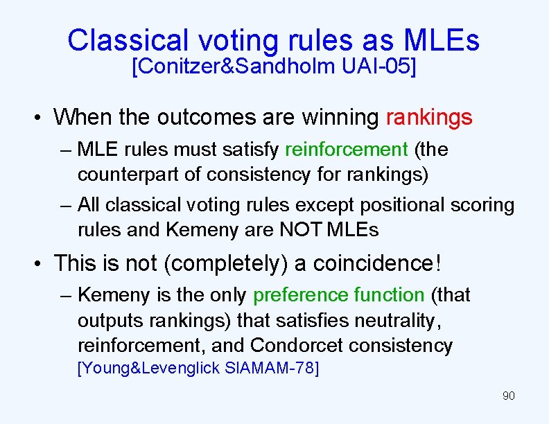
Classical voting rules as MLEs [Conitzer&Sandholm UAI-05] • When the outcomes are winning rankings – MLE rules must satisfy reinforcement (the counterpart of consistency for rankings) – All classical voting rules except positional scoring rules and Kemeny are NOT MLEs • This is not (completely) a coincidence! – Kemeny is the only preference function (that outputs rankings) that satisfies neutrality, reinforcement, and Condorcet consistency [Young&Levenglick SIAMAM-78] 90

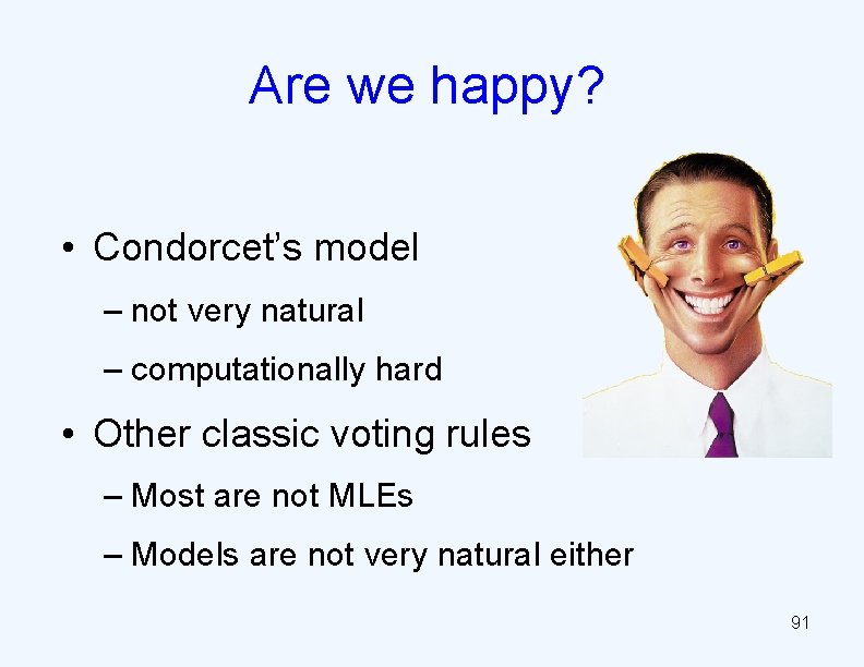
Are we happy? • Condorcet’s model – not very natural – computationally hard • Other classic voting rules – Most are not MLEs – Models are not very natural either 91

New mechanisms via the statistical decision framework Decision Model selection – How can we evaluate fitness? • Frequentist or Bayesian? – Focus on frequentist decision making Information about the ground truth inference Data D • Computation – How can we compute MLE efficiently? 92

Why not just a problem of machine learning or statistics? • Closely related, but – We need economic insight to build the model – We care about satisfaction of traditional social choice criteria • Also want to reach a compromise (achieve democracy) 93

Outline: statistical approaches Condorcet’s MLE model (history) Why MLE? Why Condorcet’s model? A General framework Random Utility Models 94

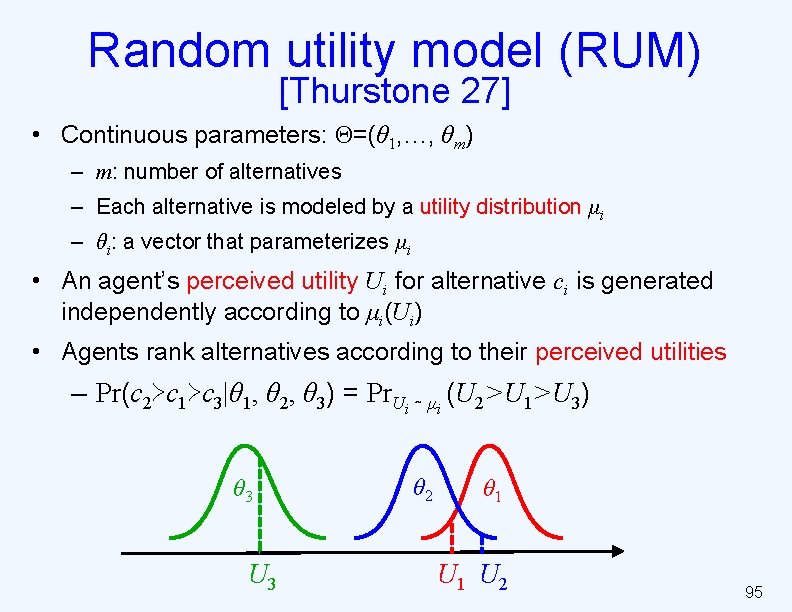
Random utility model (RUM) [Thurstone 27] • Continuous parameters: Θ=(θ 1, …, θm) – m: number of alternatives – Each alternative is modeled by a utility distribution μi – θi: a vector that parameterizes μi • An agent’s perceived utility Ui for alternative ci is generated independently according to μi(Ui) • Agents rank alternatives according to their perceived utilities – Pr(c 2≻c 1≻c 3|θ 1, θ 2, θ 3) = Pr. Ui ∼ μi (U 2>U 1>U 3) θ 3 U 3 θ 2 θ 1 U 2 95

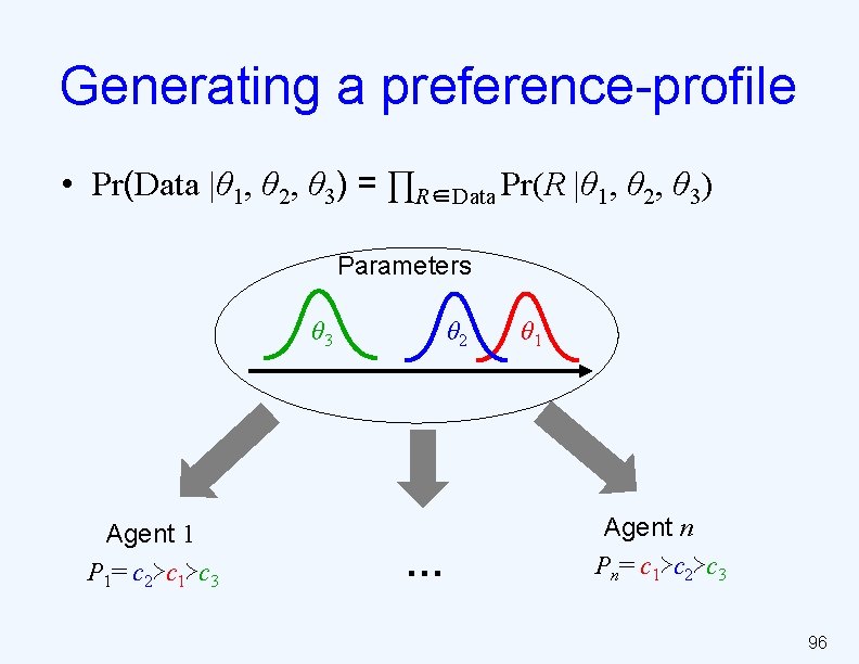
Generating a preference-profile • Pr(Data |θ 1, θ 2, θ 3) = ∏R∈Data Pr(R |θ 1, θ 2, θ 3) Parameters θ 3 Agent 1 P 1= c 2≻c 1≻c 3 θ 2 … θ 1 Agent n Pn= c 1≻c 2≻c 3 96

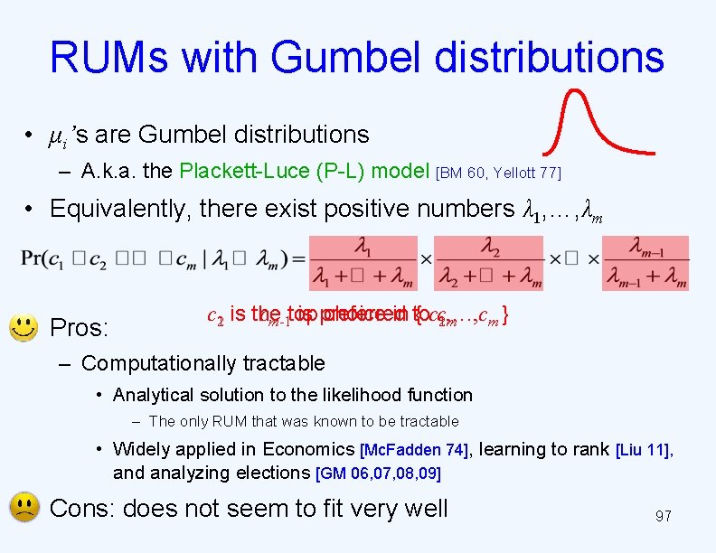
RUMs with Gumbel distributions • μi’s are Gumbel distributions – A. k. a. the Plackett-Luce (P-L) model [BM 60, Yellott 77] • Equivalently, there exist positive numbers λ 1, …, λm • Pros: c 21 is the top choice in { c cm-1 is preferred to c 21, …, c m m} – Computationally tractable • Analytical solution to the likelihood function – The only RUM that was known to be tractable • Widely applied in Economics [Mc. Fadden 74], learning to rank [Liu 11], and analyzing elections [GM 06, 07, 08, 09] • Cons: does not seem to fit very well 97

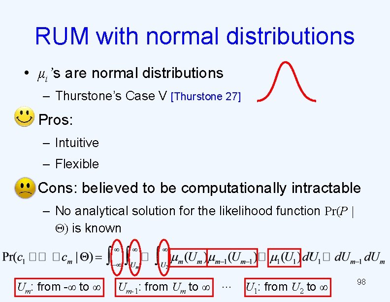
RUM with normal distributions • μi’s are normal distributions – Thurstone’s Case V [Thurstone 27] • Pros: – Intuitive – Flexible • Cons: believed to be computationally intractable – No analytical solution for the likelihood function Pr(P | Θ) is known Um: from -∞ to ∞ Um-1: from Um to ∞ … U 1: from U 2 to ∞ 98

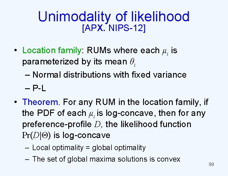
Unimodality of likelihood [APX. NIPS-12] • Location family: RUMs where each μi is parameterized by its mean θi – Normal distributions with fixed variance – P-L • Theorem. For any RUM in the location family, if the PDF of each μi is log-concave, then for any preference-profile D, the likelihood function Pr(D|Θ) is log-concave – Local optimality = global optimality – The set of global maxima solutions is convex 99

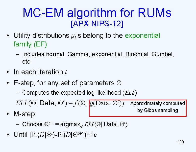
MC-EM algorithm for RUMs [APX NIPS-12] • Utility distributions μl’s belong to the exponential family (EF) – Includes normal, Gamma, exponential, Binomial, Gumbel, etc. • In each iteration t • E-step, for any set of parameters Θ – Computes the expected log likelihood (ELL) ELL(Θ| Data, Θt) = f (Θ, g(Data, Θt)) • M-step Approximately computed by Gibbs sampling – Choose Θt+1 = argmaxΘ ELL(Θ| Data, Θt) • Until |Pr(D|Θt)-Pr(D|Θt+1)|< ε 100

Outline: statistical approaches Condorcet’s MLE model (history) Why MLE? Why Condorcet’s model? A General framework Random Utility Models Model selection 101

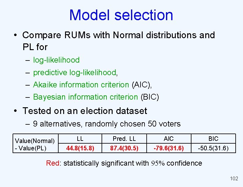
Model selection • Compare RUMs with Normal distributions and PL for – log-likelihood – predictive log-likelihood, – Akaike information criterion (AIC), – Bayesian information criterion (BIC) • Tested on an election dataset – 9 alternatives, randomly chosen 50 voters Value(Normal) - Value(PL) LL Pred. LL AIC BIC 44. 8(15. 8) 87. 4(30. 5) -79. 6(31. 6) -50. 5(31. 6) Red: statistically significant with 95% confidence 102

Recent progress • Generalized RUM [APX UAI-13] – Learn the relationship between agent features and alternative features • Preference elicitation based on experimental design [APX UAI-13] – c. f. active learning • Faster algorithms [ACPX, ACP in submission] – Generalized Method of Moments (GMM) 103

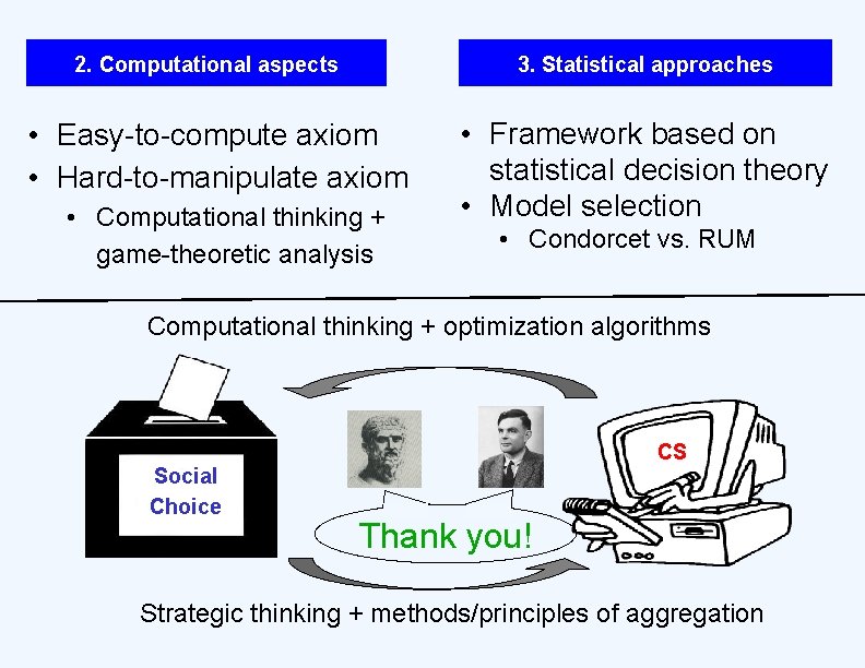
2. Computational aspects 3. Statistical approaches • Easy-to-compute axiom • Hard-to-manipulate axiom • Computational thinking + game-theoretic analysis • Framework based on statistical decision theory • Model selection • Condorcet vs. RUM Computational thinking + optimization algorithms Social Choice CS Thank you! Strategic thinking + methods/principles of aggregation