Chapter 9 Estimating the Value of a Parameter
- Slides: 27

Chapter 9 Estimating the Value of a Parameter Using Confidence Intervals © 2010 Pearson Prentice Hall. All rights reserved

Section 9. 2 Confidence Intervals about a Population Mean When the Population Standard Deviation is Unknown © 2010 Pearson Prentice Hall. All rights reserved

Objectives 1. Know the properties of Student’s t-distribution 2. Determine t-values 3. Construct and interpret a confidence interval for a population mean © 2010 Pearson Prentice Hall. All rights reserved 9 -3

Objective 1 • Know the Properties of Student’s t-Distribution © 2010 Pearson Prentice Hall. All rights reserved 9 -4

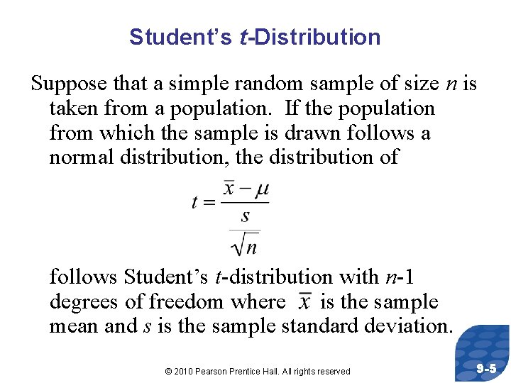
Student’s t-Distribution Suppose that a simple random sample of size n is taken from a population. If the population from which the sample is drawn follows a normal distribution, the distribution of follows Student’s t-distribution with n-1 degrees of freedom where is the sample mean and s is the sample standard deviation. © 2010 Pearson Prentice Hall. All rights reserved 9 -5

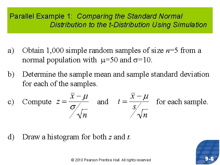
Parallel Example 1: Comparing the Standard Normal Distribution to the t-Distribution Using Simulation a) Obtain 1, 000 simple random samples of size n=5 from a normal population with =50 and =10. b) Determine the sample mean and sample standard deviation for each of the samples. c) Compute and for each sample. d) Draw a histogram for both z and t. © 2010 Pearson Prentice Hall. All rights reserved 9 -6

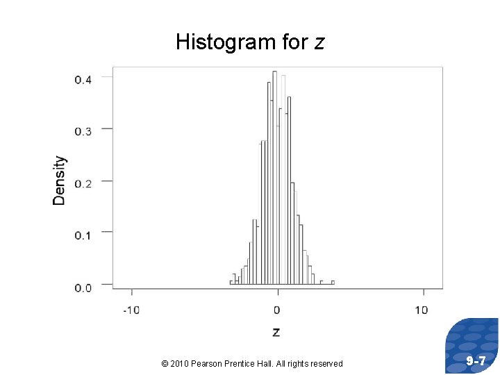
Histogram for z © 2010 Pearson Prentice Hall. All rights reserved 9 -7

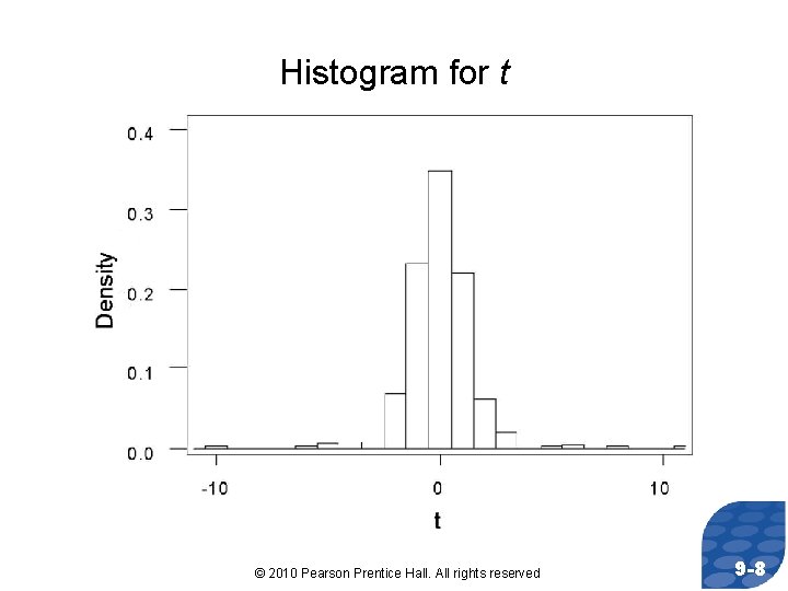
Histogram for t © 2010 Pearson Prentice Hall. All rights reserved 9 -8

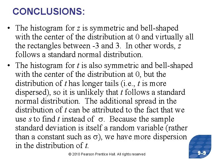
CONCLUSIONS: • The histogram for z is symmetric and bell-shaped with the center of the distribution at 0 and virtually all the rectangles between -3 and 3. In other words, z follows a standard normal distribution. • The histogram for t is also symmetric and bell-shaped with the center of the distribution at 0, but the distribution of t has longer tails (i. e. , t is more dispersed), so it is unlikely that t follows a standard normal distribution. The additional spread in the distribution of t can be attributed to the fact that we use s to find t instead of . Because the sample standard deviation is itself a random variable (rather than a constant such as ), we have more dispersion in the distribution of t. © 2010 Pearson Prentice Hall. All rights reserved 9 -9

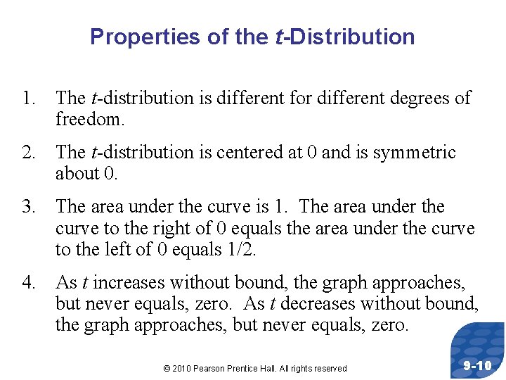
Properties of the t-Distribution 1. The t-distribution is different for different degrees of freedom. 2. The t-distribution is centered at 0 and is symmetric about 0. 3. The area under the curve is 1. The area under the curve to the right of 0 equals the area under the curve to the left of 0 equals 1/2. 4. As t increases without bound, the graph approaches, but never equals, zero. As t decreases without bound, the graph approaches, but never equals, zero. © 2010 Pearson Prentice Hall. All rights reserved 9 -10

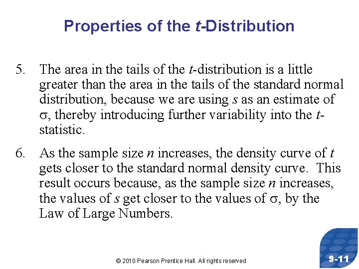
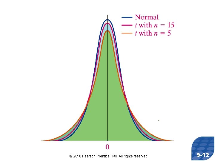
Properties of the t-Distribution 5. The area in the tails of the t-distribution is a little greater than the area in the tails of the standard normal distribution, because we are using s as an estimate of , thereby introducing further variability into the tstatistic. 6. As the sample size n increases, the density curve of t gets closer to the standard normal density curve. This result occurs because, as the sample size n increases, the values of s get closer to the values of , by the Law of Large Numbers. © 2010 Pearson Prentice Hall. All rights reserved 9 -11

© 2010 Pearson Prentice Hall. All rights reserved 9 -12

Objective 2 • Determine t-Values © 2010 Pearson Prentice Hall. All rights reserved 9 -13

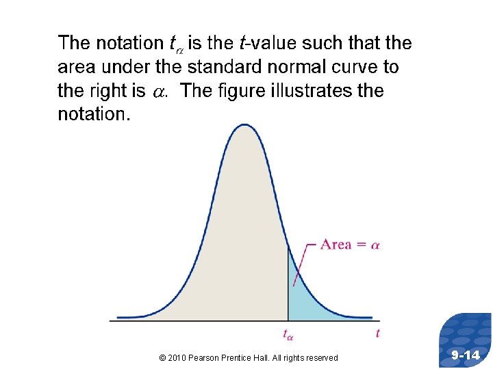
© 2010 Pearson Prentice Hall. All rights reserved 9 -14

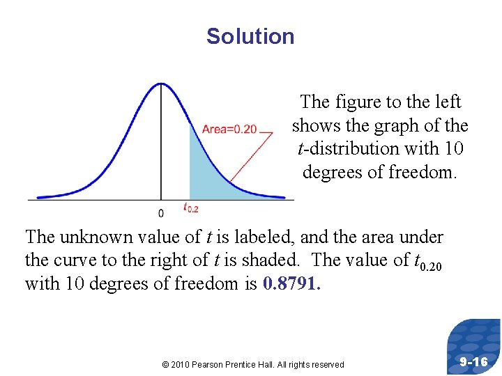
Parallel Example 2: Finding t-values Find the t-value such that the area under the tdistribution to the right of the t-value is 0. 2 assuming 10 degrees of freedom. That is, find t 0. 20 with 10 degrees of freedom. © 2010 Pearson Prentice Hall. All rights reserved 9 -15

Solution The figure to the left shows the graph of the t-distribution with 10 degrees of freedom. The unknown value of t is labeled, and the area under the curve to the right of t is shaded. The value of t 0. 20 with 10 degrees of freedom is 0. 8791. © 2010 Pearson Prentice Hall. All rights reserved 9 -16

Objective 3 • Construct and Interpret a Confidence Interval for a Population Mean © 2010 Pearson Prentice Hall. All rights reserved 9 -17

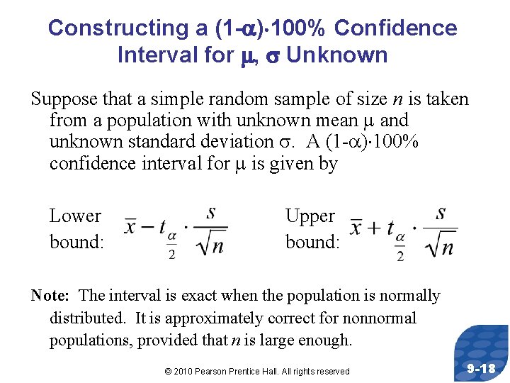
Constructing a (1 - ) 100% Confidence Interval for , Unknown Suppose that a simple random sample of size n is taken from a population with unknown mean and unknown standard deviation . A (1 - ) 100% confidence interval for is given by Lower bound: Upper bound: Note: The interval is exact when the population is normally distributed. It is approximately correct for nonnormal populations, provided that n is large enough. © 2010 Pearson Prentice Hall. All rights reserved 9 -18

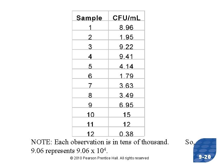
Parallel Example 3: Constructing a Confidence Interval about a Population Mean The pasteurization process reduces the amount of bacteria found in dairy products, such as milk. The following data represent the counts of bacteria in pasteurized milk (in CFU/m. L) for a random sample of 12 pasteurized glasses of milk. Data courtesy of Dr. Michael Lee, Professor, Joliet Junior College. Construct a 95% confidence interval for the bacteria count. © 2010 Pearson Prentice Hall. All rights reserved 9 -19

NOTE: Each observation is in tens of thousand. 9. 06 represents 9. 06 x 104. © 2010 Pearson Prentice Hall. All rights reserved So, 9 -20

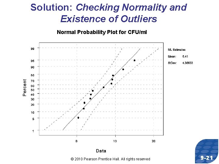
Solution: Checking Normality and Existence of Outliers Normal Probability Plot for CFU/ml © 2010 Pearson Prentice Hall. All rights reserved 9 -21

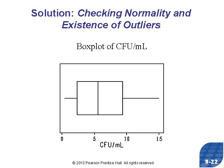
Solution: Checking Normality and Existence of Outliers Boxplot of CFU/m. L © 2010 Pearson Prentice Hall. All rights reserved 9 -22

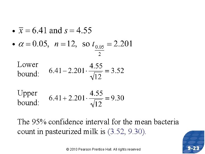
• • Lower bound: Upper bound: The 95% confidence interval for the mean bacteria count in pasteurized milk is (3. 52, 9. 30). © 2010 Pearson Prentice Hall. All rights reserved 9 -23

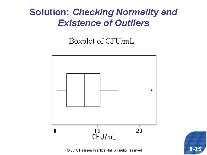
Parallel Example 5: The Effect of Outliers Suppose a student miscalculated the amount of bacteria and recorded a result of 2. 3 x 10⁵. We would include this value in the data set as 23. 0. What effect does this additional observation have on the 95% confidence interval? © 2010 Pearson Prentice Hall. All rights reserved 9 -24

Solution: Checking Normality and Existence of Outliers Boxplot of CFU/m. L © 2010 Pearson Prentice Hall. All rights reserved 9 -25

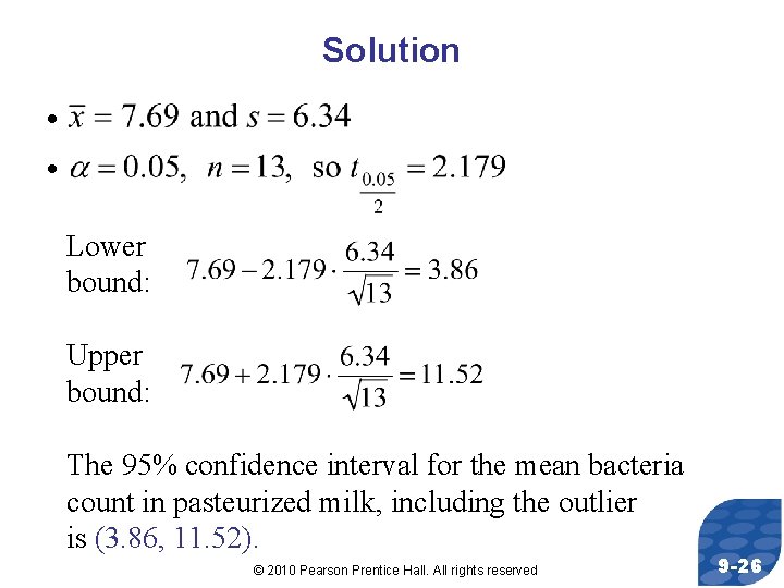
Solution • • Lower bound: Upper bound: The 95% confidence interval for the mean bacteria count in pasteurized milk, including the outlier is (3. 86, 11. 52). © 2010 Pearson Prentice Hall. All rights reserved 9 -26

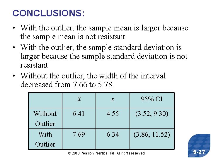
CONCLUSIONS: • With the outlier, the sample mean is larger because the sample mean is not resistant • With the outlier, the sample standard deviation is larger because the sample standard deviation is not resistant • Without the outlier, the width of the interval decreased from 7. 66 to 5. 78. s 95% CI Without Outlier 6. 41 4. 55 (3. 52, 9. 30) With Outlier 7. 69 6. 34 (3. 86, 11. 52) © 2010 Pearson Prentice Hall. All rights reserved 9 -27