Estimating the Value of a Parameter Using Confidence

Estimating the Value of a Parameter Using Confidence Intervals Prof. L Prado www. helpyourmath. com 1

Inferential Statistics • 1. Involves: Population? – Estimation – Hypothesis Testing • 2. Purpose – Make Decisions about Population Characteristics 2

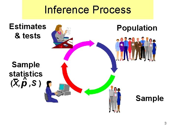
Inference Process Estimates & tests Population Sample statistics ^ , S ) (X, p Sample 3

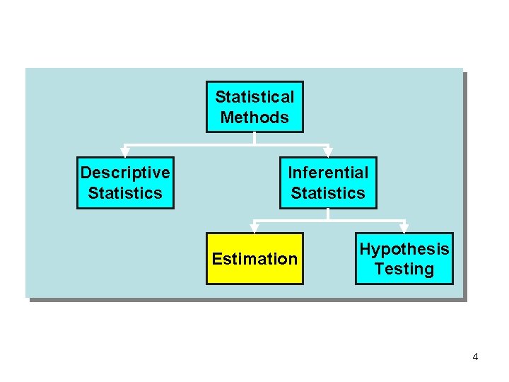
Statistical Methods Descriptive Statistics Inferential Statistics Estimation Hypothesis Testing 4

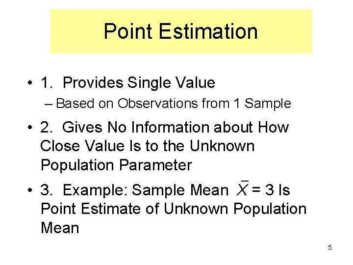
Point Estimation • 1. Provides Single Value – Based on Observations from 1 Sample • 2. Gives No Information about How Close Value Is to the Unknown Population Parameter • 3. Example: Sample Mean X = 3 Is Point Estimate of Unknown Population Mean 5

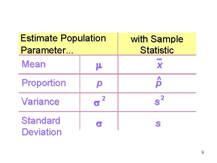
Estimate Population Parameter. . . Mean Proportion p 2 Variance Standard Deviation with Sample Statistic x p^ s 2 s 6

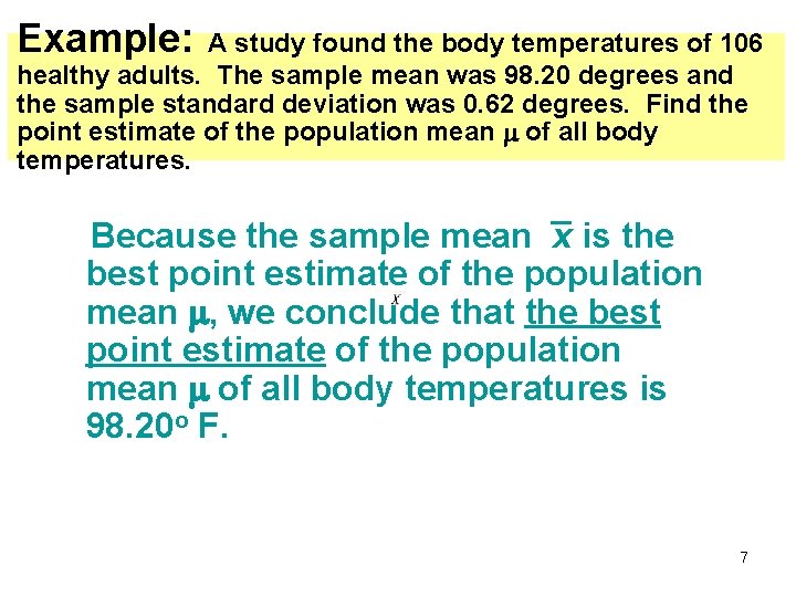
Example: A study found the body temperatures of 106 healthy adults. The sample mean was 98. 20 degrees and the sample standard deviation was 0. 62 degrees. Find the point estimate of the population mean of all body temperatures. Because the sample mean x is the best point estimate of the population mean , we conclude that the best point estimate of the population mean of all body temperatures is 98. 20 o F. 7

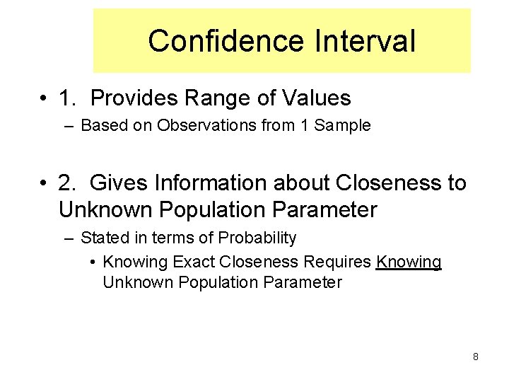
Confidence Interval • 1. Provides Range of Values – Based on Observations from 1 Sample • 2. Gives Information about Closeness to Unknown Population Parameter – Stated in terms of Probability • Knowing Exact Closeness Requires Knowing Unknown Population Parameter 8

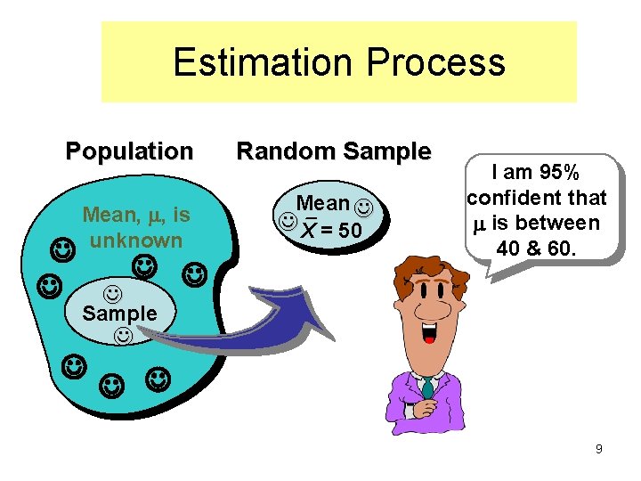
Estimation Process Population Mean, , is unknown Random Sample Mean X = 50 I am 95% confident that is between 40 & 60. Sample 9

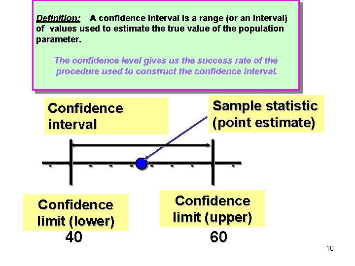
Definition: A confidence interval is a range (or an interval) of values used to estimate the true value of the population parameter. The confidence level gives us the success rate of the procedure used to construct the confidence interval. Confidence interval Confidence limit (lower) 40 Sample statistic (point estimate) Confidence limit (upper) 60 10

Confidence Intervals • Learning objectives 1 – Compute a point estimate of the population proportion 2 – Construct and interpret a confidence interval about the population proportion 3 – Understand the role of margin of error in constructing a confidence interval 11

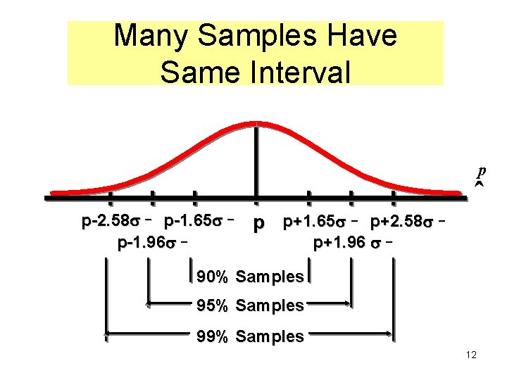
Many Samples Have Same Interval p p-2. 58 p-1. 65 p-1. 96 ˆ p p+1. 65 p+2. 58 p+1. 96 90% Samples 95% Samples 99% Samples 12

Chapter 7 – Section 1 • Learning objectives – Obtain a point estimate for the population proportion 2 – Construct and interpret a confidence interval for the population proportion 3 – Determine the sample size necessary for estimating a population proportion within a specified margin of error 1 13

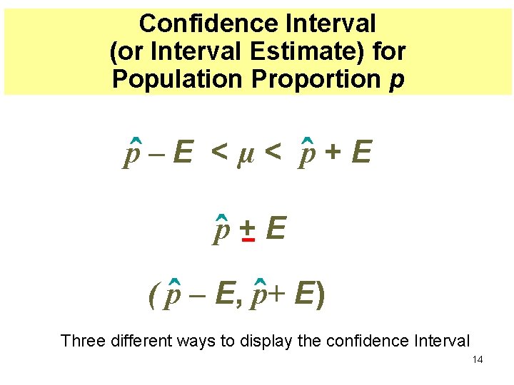
Confidence Interval (or Interval Estimate) for Population Proportion p pˆ – E < µ < pˆ + E ( pˆ – E, p+ ˆ E) Three different ways to display the confidence Interval 14

• We have already studied the distribution of the sample proportion is approximately normal with under most conditions • We use this to construct confidence intervals for the population proportion 15

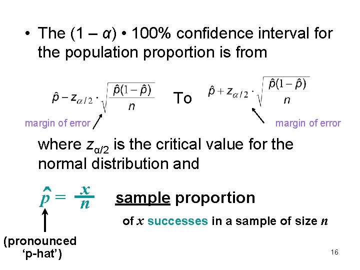
• The (1 – α) • 100% confidence interval for the population proportion is from To margin of error where zα/2 is the critical value for the normal distribution and x pˆ = n sample proportion of x successes in a sample of size n (pronounced ‘p-hat’) 16

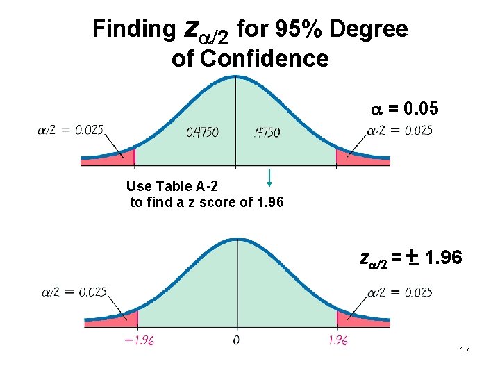
Finding z 2 for 95% Degree of Confidence = 0. 05 Use Table A-2 to find a z score of 1. 96 z 2 = 1. 96 17

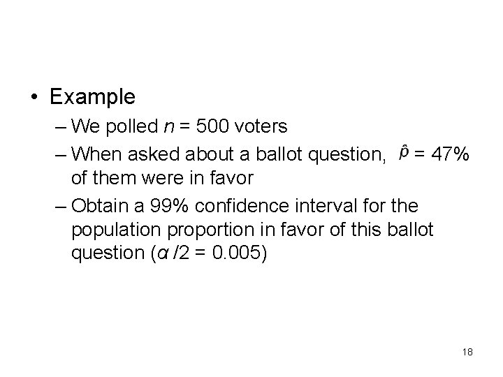
• Example – We polled n = 500 voters – When asked about a ballot question, = 47% of them were in favor – Obtain a 99% confidence interval for the population proportion in favor of this ballot question (α /2 = 0. 005) 18

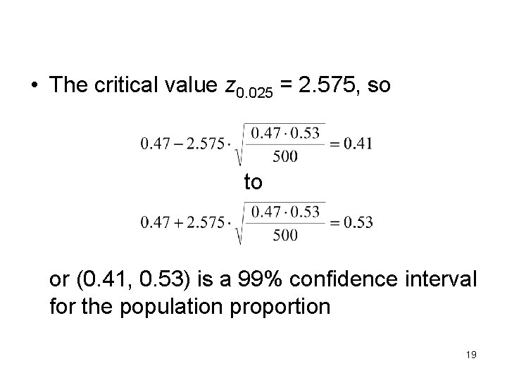
• The critical value z 0. 025 = 2. 575, so to or (0. 41, 0. 53) is a 99% confidence interval for the population proportion 19

Summary: Chapter 7 – Section 1 • We can construct confidence intervals for population proportions in much the same way as for population means • We need to use the formula for the standard deviation of the sample proportion • We can also compute the minimum sample size for a desired level of accuracy 20

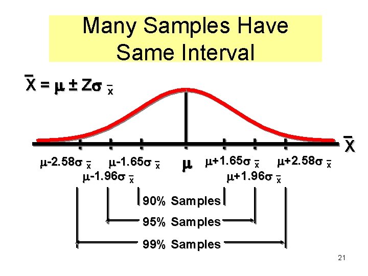
Many Samples Have Same Interval X = ± Z x -2. 58 x -1. 65 x -1. 96 x +1. 65 x +2. 58 x +1. 96 x X 90% Samples 95% Samples 99% Samples 21

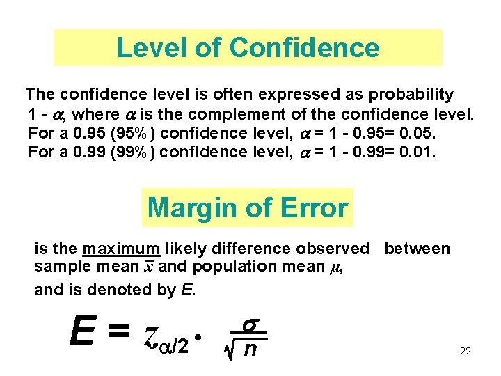
Level of Confidence The confidence level is often expressed as probability 1 - , where is the complement of the confidence level. For a 0. 95 (95%) confidence level, = 1 - 0. 95= 0. 05. For a 0. 99 (99%) confidence level, = 1 - 0. 99= 0. 01. Margin of Error is the maximum likely difference observed between sample mean x and population mean µ, and is denoted by E. E = z /2 • n 22

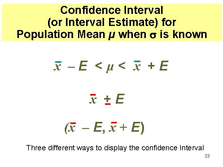
Confidence Interval (or Interval Estimate) for Population Mean µ when is known x –E <µ< x +E (x – E, x + E) Three different ways to display the confidence Interval 23

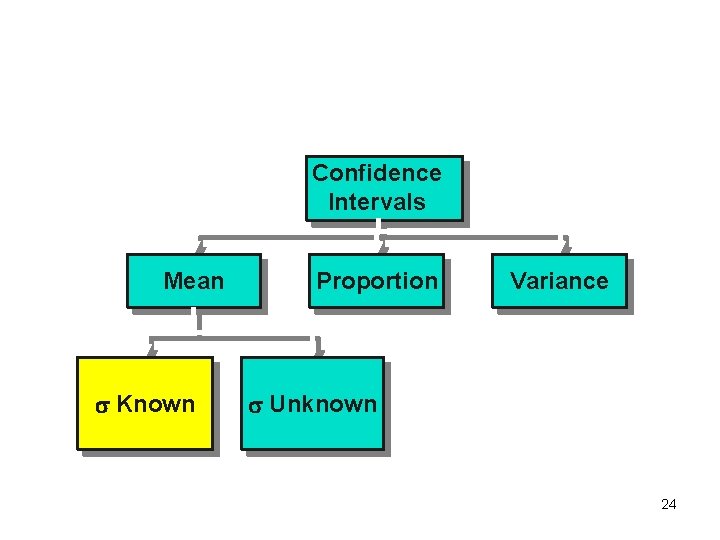
Confidence Intervals Mean Known Proportion Variance Unknown 24

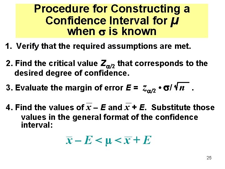
Procedure for Constructing a Confidence Interval for µ when is known 1. Verify that the required assumptions are met. 2. Find the critical value z 2 that corresponds to the desired degree of confidence. 3. Evaluate the margin of error E = z 2 • / n . 4. Find the values of x – E and x + E. Substitute those values in the general format of the confidence interval: x–E<µ<x+E 25

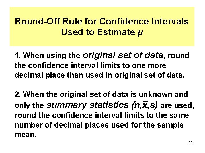
Round-Off Rule for Confidence Intervals Used to Estimate µ 1. When using the original set of data, round the confidence interval limits to one more decimal place than used in original set of data. 2. When the original set of data is unknown and only the summary statistics (n, x, s) are used, round the confidence interval limits to the same number of decimal places used for the sample mean. 26

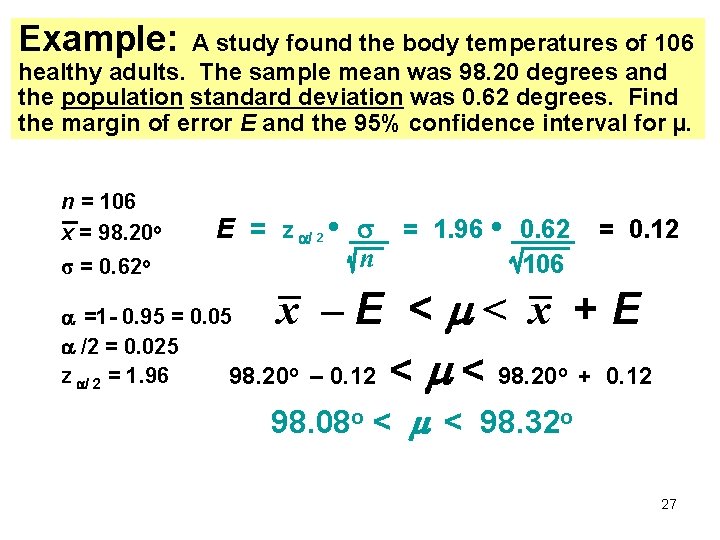
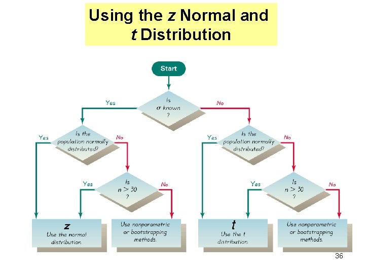
Example: A study found the body temperatures of 106 healthy adults. The sample mean was 98. 20 degrees and the population standard deviation was 0. 62 degrees. Find the margin of error E and the 95% confidence interval for µ. n = 106 x = 98. 20 o σ = 0. 62 o E = z / 2 • n = 1. 96 • 0. 62 106 = 0. 12 x –E < < x +E =1 - 0. 95 = 0. 05 /2 = 0. 025 z / 2 = 1. 96 98. 20 o – 0. 12 < < 98. 20 o + 0. 12 98. 08 o < < 98. 32 o 27

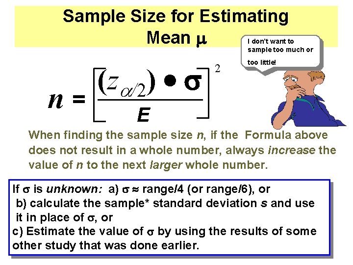
Sample Size for Estimating Mean I don’t want to sample too much or n= (z /2) 2 too little! E When finding the sample size n, if the Formula above does not result in a whole number, always increase the value of n to the next larger whole number. If is unknown: a) range/4 (or range/6), or b) calculate the sample* standard deviation s and use it in place of , or c) Estimate the value of by using the results of some other study that was done earlier. 28

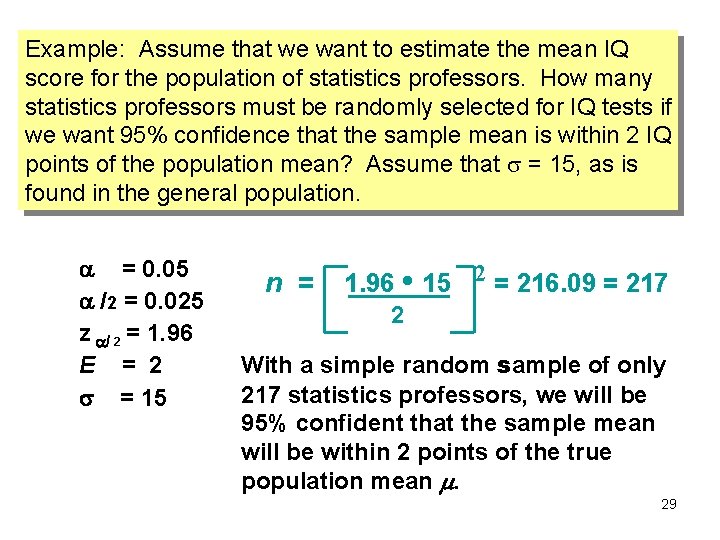
Example: Assume that we want to estimate the mean IQ score for the population of statistics professors. How many statistics professors must be randomly selected for IQ tests if we want 95% confidence that the sample mean is within 2 IQ points of the population mean? Assume that = 15, as is found in the general population. = 0. 05 /2 = 0. 025 z / 2 = 1. 96 E = 2 = 15 n = 1. 96 • 15 2 = 216. 09 = 217 2 With a simple random sample of only 217 statistics professors, we will be 95% confident that the sample mean will be within 2 points of the true population mean . 29

Summary • We can construct a confidence interval around a point estimator if we know the population standard deviation σ • The margin of error is calculated using σ, the sample size n, and the appropriate Zvalue • We can also calculate the sample size needed to obtain a target margin of error 30

Learning Objectives – Know the properties of t-distribution 2 – Determine t-values 3 – Construct and interpret a confidence interval about a population mean 1 31

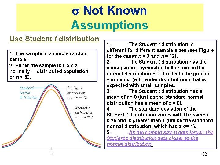
Not Known Assumptions Use Student t distribution 1) The sample is a simple random sample. 2) Either the sample is from a normally distributed population, or n > 30. 1. The Student t distribution is different for different sample sizes (see Figure for the cases n = 3 and n = 12). 2. The Student t distribution has the same general symmetric bell shape as the normal distribution but it reflects the greater variability (with wider distributions) that is expected with small samples. 3. The Student t distribution has a mean of t = 0 (just as the standard normal distribution has a mean of z = 0). 4. The standard deviation of the Student t distribution varies with the sample size and is greater than 1 (unlike the standard normal distribution, which has a σ= 1). 5. As the sample size n gets larger, the Student t distribution gets closer to the normal distribution. 32

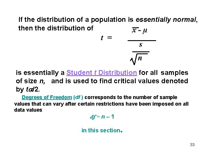
If the distribution of a population is essentially normal, then the distribution of x-µ t = s n is essentially a Student t Distribution for all samples of size n, and is used to find critical values denoted by t /2. Degrees of Freedom (df ) corresponds to the number of sample values that can vary after certain restrictions have been imposed on all data values df = n – 1 in this section . 33

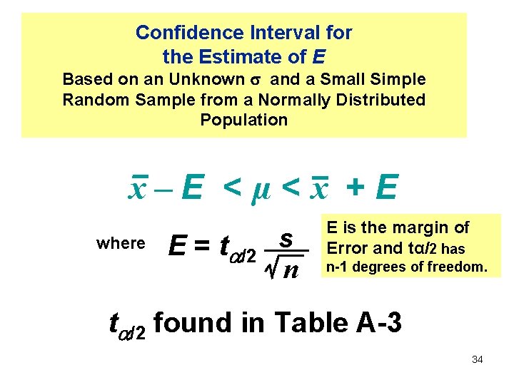
Confidence Interval for the Estimate of E Based on an Unknown and a Small Simple Random Sample from a Normally Distributed Population x–E <µ<x +E where E = t /2 s n E is the margin of Error and tα/2 has n-1 degrees of freedom. t /2 found in Table A-3 34

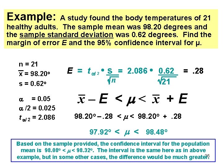
Example: A study found the body temperatures of 21 healthy adults. The sample mean was 98. 20 degrees and the sample standard deviation was 0. 62 degrees. Find the margin of error E and the 95% confidence interval for µ. n = 21 x = 98. 20 o s = 0. 62 o = 0. 05 /2 = 0. 025 t / 2 = 2. 086 E = t / 2 • s = 2. 086 • 0. 62 n 21 =. 28 x–E < < x +E 98. 20 o –. 28 < < 98. 20 o +. 28 97. 92 o < < 98. 48 o Based on the sample provided, the confidence interval for the population mean is 98. 08 o < < 98. 32 o. The interval is the same here as in above 35 example, but in some other cases, the difference would be much greater.

Using the z Normal and t Distribution 36

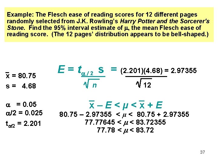
Example: The Flesch ease of reading scores for 12 different pages randomly selected from J. K. Rowling’s Harry Potter and the Sorcerer’s Stone. Find the 95% interval estimate of , the mean Flesch ease of reading score. (The 12 pages’ distribution appears to be bell-shaped. ) x = 80. 75 s = 4. 68 = 0. 05 /2 = 0. 025 t /2 = 2. 201 E = t 2 s = n (2. 201)(4. 68) = 2. 97355 12 x–E<µ<x+E 80. 75 – 2. 97355 < µ < 80. 75 + 2. 97355 77. 77645 < < 83. 72355 77. 78 < < 83. 72 37