Chapter 15 1 15 1 Random Experiments and

Chapter 15 -1 15. 1 Random Experiments and Sample Spaces 15. 2 Counting Outcomes in Sample Spaces 15. 3 Permutations and Combinations 15. 4 Probability Spaces 15. 5 Equiprobable Spaces 15. 6 Odds Copyright © 2010 Pearson Education, Inc. Excursions in Modern Mathematics, 7 e: 15. 1 - 1

Random Experiment In broad terms, probability is the quantification of uncertainty. To understand what that means, we may start by formalizing the notion of uncertainty. We will use the term random experiment to describe an activity or a process whose outcome cannot be predicted ahead of time. Typical examples of random experiments are tossing a coin, rolling a pair of dice, drawing cards out of a deck of cards, predicting the result of a football game, and forecasting the path of a hurricane. Copyright © 2010 Pearson Education, Inc. Excursions in Modern Mathematics, 7 e: 15. 1 - 2

Sample Space Associated with every random experiment is the set of all of its possible outcomes, called the sample space of the experiment. For the sake of simplicity, we will concentrate on experiments for which there is only a finite set of outcomes, although experiments with infinitely many outcomes are both possible and important. Copyright © 2010 Pearson Education, Inc. Excursions in Modern Mathematics, 7 e: 15. 1 - 3

Sample Space - Set Notation Since the sample space of any experiment is a set of outcomes, we will use set notation to describe it. We will consistently use the letter S to denote a sample space and the letter N to denote the size of the sample space S (i. e. , the number of outcomes in S). Copyright © 2010 Pearson Education, Inc. Excursions in Modern Mathematics, 7 e: 15. 1 - 4

Example 15. 1 Tossing a Coin One simple random experiment is to toss a quarter and observe whether it lands heads or tails. The sample space can be described by S = {H, T}, where H stands for Heads and T for Tails. Here N = 2. Copyright © 2010 Pearson Education, Inc. Excursions in Modern Mathematics, 7 e: 15. 1 - 5

Example 15. 2 More Coin Tossing Suppose we toss a coin twice and record the outcome of each toss (H or T) in the order it happens. The sample space now is S = {HH, HT, TH, TT}, where HT means that the first toss came up H and the second toss came up T, which is a different outcome from TH (first toss T and second toss H). In this sample space N = 4. Copyright © 2010 Pearson Education, Inc. Excursions in Modern Mathematics, 7 e: 15. 1 - 6

Example 15. 2 More Coin Tossing Suppose now we toss two distinguishable coins (say, a nickel and a quarter) at the same time (tricky but definitely possible). This random experiment appears different from the one where we toss one coin twice, but the sample space is still S = {HH, HT, TH, TT}. (Here we must agree what the order of the symbols is–for example, the first symbol describes the quarter and the second the nickel. ) Copyright © 2010 Pearson Education, Inc. Excursions in Modern Mathematics, 7 e: 15. 1 - 7

Example 15. 2 More Coin Tossing Since they have the sample space, we will consider the two random experiments just described as the same random experiment. Now let’s consider a different random experiment. We are still tossing a coin twice, but we only care now about the number of heads that come up. Here there are only three possible outcomes (no heads, one head, or both heads), and symbolically we might describe this sample space as S = {0, 1, 2}. Copyright © 2010 Pearson Education, Inc. Excursions in Modern Mathematics, 7 e: 15. 1 - 8

Example 15. 3 Shooting Free Throws Here is a familiar scenario: Your favorite basketball team is down by 1, clock running out, and one of your players is fouled and goes to the line to shoot free throws, with the game riding on the outcome. It’s not a good time to think of sample spaces, but let’s do it anyway. Clearly the shooting of free throws is a random experiment, but what is the sample space? As in Example 15. 2, the answer depends on a few subtleties. Copyright © 2010 Pearson Education, Inc. Excursions in Modern Mathematics, 7 e: 15. 1 - 9

Example 15. 3 Shooting Free Throws In one scenario (the penalty situation) your player is going to shoot two free throws no matter what. In this case one could argue that what really matters is how many free throws he or she makes (make both and win the game, miss one and tie and go to overtime, miss both and lose the game). When we look at it this way the sample space is S = {0, 1, 2}. Copyright © 2010 Pearson Education, Inc. Excursions in Modern Mathematics, 7 e: 15. 1 - 10

Example 15. 3 Shooting Free Throws A somewhat more stressful scenario is when your player is shooting a one-and-one. This means that the player gets to shoot the second free throw only if he or she makes the first one. In this case there also three possible outcomes, but the circumstances are different because the order of events is relevant (miss the first free throw and lose the game, make the first free throw but miss the second one and tie the game, make both and win the game). Copyright © 2010 Pearson Education, Inc. Excursions in Modern Mathematics, 7 e: 15. 1 - 11

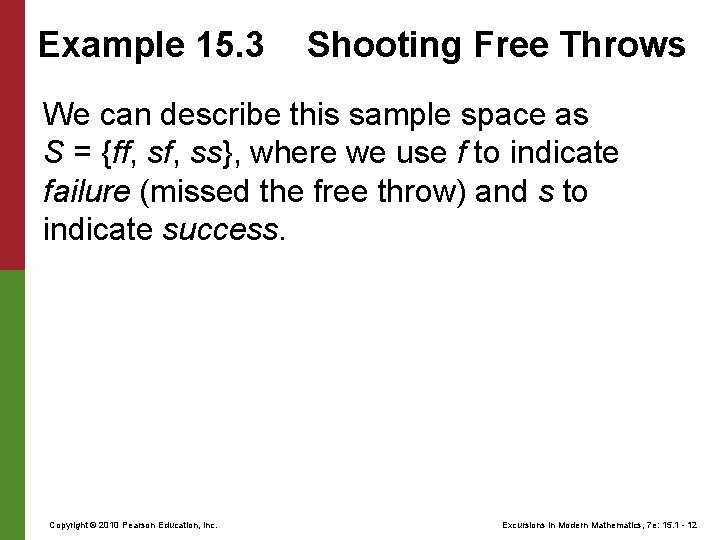
Example 15. 3 Shooting Free Throws We can describe this sample space as S = {ff, ss}, where we use f to indicate failure (missed the free throw) and s to indicate success. Copyright © 2010 Pearson Education, Inc. Excursions in Modern Mathematics, 7 e: 15. 1 - 12

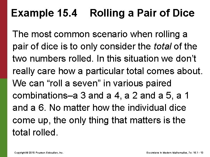
Example 15. 4 Rolling a Pair of Dice The most common scenario when rolling a pair of dice is to only consider the total of the two numbers rolled. In this situation we don’t really care how a particular total comes about. We can “roll a seven” in various paired combinations–a 3 and a 4, a 2 and a 5, a 1 and a 6. No matter how the individual dice come up, the only thing that matters is the total rolled. Copyright © 2010 Pearson Education, Inc. Excursions in Modern Mathematics, 7 e: 15. 1 - 13

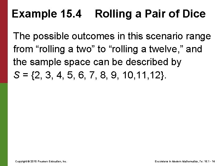
Example 15. 4 Rolling a Pair of Dice The possible outcomes in this scenario range from “rolling a two” to “rolling a twelve, ” and the sample space can be described by S = {2, 3, 4, 5, 6, 7, 8, 9, 10, 11, 12}. Copyright © 2010 Pearson Education, Inc. Excursions in Modern Mathematics, 7 e: 15. 1 - 14

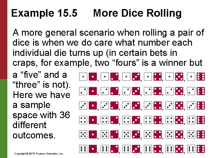
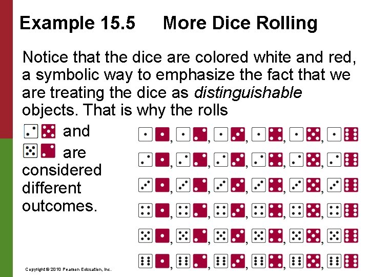
Example 15. 5 More Dice Rolling A more general scenario when rolling a pair of dice is when we do care what number each individual die turns up (in certain bets in craps, for example, two “fours” is a winner but a “five” and a “three” is not). Here we have a sample space with 36 different outcomes. Copyright © 2010 Pearson Education, Inc. Excursions in Modern Mathematics, 7 e: 15. 1 - 15

Example 15. 5 More Dice Rolling Notice that the dice are colored white and red, a symbolic way to emphasize the fact that we are treating the dice as distinguishable objects. That is why the rolls and are considered different outcomes. Copyright © 2010 Pearson Education, Inc. Excursions in Modern Mathematics, 7 e: 15. 1 - 16

Example 15. 6 More Dice Rolling Five candidates (A, B, C, D, and E) are running in an election. The top three vote getters are chosen President, Vice President, and Secretary, in that order. Such an election can be considered a random experiment with sample space S = {ABC, ACB, BAC, BCA, CAB, CBA, ABD, ADB, …, CDE}. We will assume that outcome ABC denotes that candidate A is elected President, B is elected Vice President, and C is elected Secretary. Copyright © 2010 Pearson Education, Inc. Excursions in Modern Mathematics, 7 e: 15. 1 - 17

Example 15. 6 More Dice Rolling This is important because the outcomes ABC and BAC are different outcomes and must appear separately in the sample space. Because this sample space is a bit too large to write out in full (we will soon learn that its size is N = 60), we use the “. . . ” notation. It is a way of saying “and so on–you get the point. ” Copyright © 2010 Pearson Education, Inc. Excursions in Modern Mathematics, 7 e: 15. 1 - 18

Not Listing All of the Outcomes Example 15. 6 illustrates the point that sample spaces can have a lot of outcomes and that we are often justified in not writing each and every one of them down. This is where the “. . . ” comes in handy. The key thing is to understand what the sample space looks like without necessarily writing all the outcomes down. Our real goal is to find N, the size of the sample space. If we can do it without having to list all the outcomes, then so much the better. Copyright © 2010 Pearson Education, Inc. Excursions in Modern Mathematics, 7 e: 15. 1 - 19

Chapter 15 - 2 15. 1 Random Experiments and Sample Spaces 15. 2 Counting Outcomes in Sample Spaces 15. 3 Permutations and Combinations 15. 4 Probability Spaces 15. 5 Equiprobable Spaces 15. 6 Odds Copyright © 2010 Pearson Education, Inc. Excursions in Modern Mathematics, 7 e: 15. 1 - 20

Example 15. 7 Tossing More Coins If we toss a coin three times and separately record the outcome of each toss, the sample space is given by S = {HHH, HHT, HTH, HTT, THH, THT, TTH, TTT}. Here we can just count the outcomes and get N = 8. Now let’s look at an expanded version of the same idea and toss a coin 10 times (and record the outcome of each toss). In this case the sample space S is too big to write down, but we can “count” the number of outcomes in S without having to tally them one by one. Here is how we do it. Copyright © 2010 Pearson Education, Inc. Excursions in Modern Mathematics, 7 e: 15. 1 - 21

Example 15. 7 Tossing More Coins Each outcome in S can be described by a string of 10 consecutive letters, where each letter is either H or T. (This is a natural extension of the ideas introduced in Example 15. 2. ) For example, THHTHTHHTT represents a single outcome in our sample space–the one in which the first toss came up T, the second toss came up H, the third toss came up H, and so on. Copyright © 2010 Pearson Education, Inc. Excursions in Modern Mathematics, 7 e: 15. 1 - 22

Example 15. 7 Tossing More Coins To count all the outcomes, we will argue as follows: There are two choices for the first letter (H or T), two choices for the second letter, two choices for the third letter, and so on down to the tenth letter. The total number of possible strings is found by multiplying the number of choices for each letter. Thus N = 210 = 1024. Copyright © 2010 Pearson Education, Inc. Excursions in Modern Mathematics, 7 e: 15. 1 - 23

Multiplication Rule The rule we used in Example 15. 6 is an old friend from Chapter 2–the multiplication rule, and for a formal definition of the multiplication rule the reader is referred to Section 2. 4. Informally, the multiplication rule simply says that when something is done in stages, the number of ways it can be done is found by multiplying the number of ways each of the stages can be done. Copyright © 2010 Pearson Education, Inc. Excursions in Modern Mathematics, 7 e: 15. 1 - 24

Example 15. 8 The Making of a Wardrobe Dolores is a young saleswoman planning her next business trip. She is thinking about packing three different pairs of shoes, four skirts, six blouses, and two jackets. If all the items are color coordinated, how many different outfits will she be able to create by combining these items? To answer this question, we must first define what we mean by an “outfit. ” Copyright © 2010 Pearson Education, Inc. Excursions in Modern Mathematics, 7 e: 15. 1 - 25

Example 15. 8 The Making of a Wardrobe Let’s assume that an outfit consists of one pair of shoes, one skirt, one blouse, and one jacket. Then to make an outfit Dolores must choose a pair of shoes (three choices), a skirt (four choices), a blouse (six choices), and a jacket (two choices). By the multiplication rule the total number of possible outfits is 3 4 6 2 = 144. Copyright © 2010 Pearson Education, Inc. Excursions in Modern Mathematics, 7 e: 15. 1 - 26

Example 15. 9 The Making of a Wardrobe: Part 2 Once again, Dolores is packing for a business trip. This time, she packs three pairs of shoes, four skirts, three pairs of slacks, six blouses, three turtlenecks, and two jackets. As before, we can assume that she coordinates the colors so that everything goes with everything else. Copyright © 2010 Pearson Education, Inc. Excursions in Modern Mathematics, 7 e: 15. 1 - 27

Example 15. 9 The Making of a Wardrobe: Part 2 This time, we will define an outfit as consisting of a pair of shoes, a choice of “lower wear” (either a skirt or a pair of slacks), and a choice of “upper wear” (it could be a blouse or a turtleneck or both), and, finally, she may or may not choose to wear a jacket. How many different such outfits are possible? Copyright © 2010 Pearson Education, Inc. Excursions in Modern Mathematics, 7 e: 15. 1 - 28

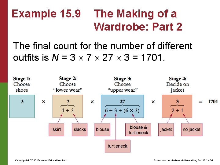
Example 15. 9 The Making of a Wardrobe: Part 2 This is a more sophisticated variation of Example 15. 8. Our strategy will be to think of an outfit as being put together in stages and to draw a box for each of the stages. We then separately count the number of choices at each stage and enter that number in the corresponding box. The last step is to multiply the numbers in each box, which we do on the next slide. Copyright © 2010 Pearson Education, Inc. Excursions in Modern Mathematics, 7 e: 15. 1 - 29

Example 15. 9 The Making of a Wardrobe: Part 2 The final count for the number of different outfits is N = 3 7 27 3 = 1701. Copyright © 2010 Pearson Education, Inc. Excursions in Modern Mathematics, 7 e: 15. 1 - 30

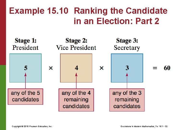
Example 15. 10 Ranking the candidate in an Election: Part 2 Five candidates are running in an election, with the top three vote getters elected (in order) as President, Vice President, and Secretary. We want to know how big the sample space is. Using a box model, we see that this becomes a reasonably easy counting problem on the next slide. Copyright © 2010 Pearson Education, Inc. Excursions in Modern Mathematics, 7 e: 15. 1 - 31

Example 15. 10 Ranking the Candidate in an Election: Part 2 Copyright © 2010 Pearson Education, Inc. Excursions in Modern Mathematics, 7 e: 15. 1 - 32

Chapter 15 - 3 15. 1 Random Experiments and Sample Spaces 15. 2 Counting Outcomes in Sample Spaces 15. 3 Permutations and Combinations 15. 4 Probability Spaces 15. 5 Equiprobable Spaces 15. 6 Odds Copyright © 2010 Pearson Education, Inc. Excursions in Modern Mathematics, 7 e: 15. 1 - 33

Counting Problems Many counting problems can be reduced to a question of counting the number of ways in which we can choose groups of objects from a larger group of objects. Often these problems require somewhat more sophisticated counting methods than the plain vanilla multiplication rule. Copyright © 2010 Pearson Education, Inc. Excursions in Modern Mathematics, 7 e: 15. 1 - 34

Counting Problems In this section we will discuss the dual concepts of permutation (a group of objects in which the ordering of the objects within the group makes a difference) and combination (a group of objects in which the ordering of the objects is irrelevant). Copyright © 2010 Pearson Education, Inc. Excursions in Modern Mathematics, 7 e: 15. 1 - 35

Example 15. 11 The Pleasures of Ice Cream Baskin-Robbins offers 31 different flavors of ice cream. A “true double” is the name we will use for two scoops of ice cream of two different flavors. Say you want a true double in a bowl–how many different choices do you have? Copyright © 2010 Pearson Education, Inc. Excursions in Modern Mathematics, 7 e: 15. 1 - 36

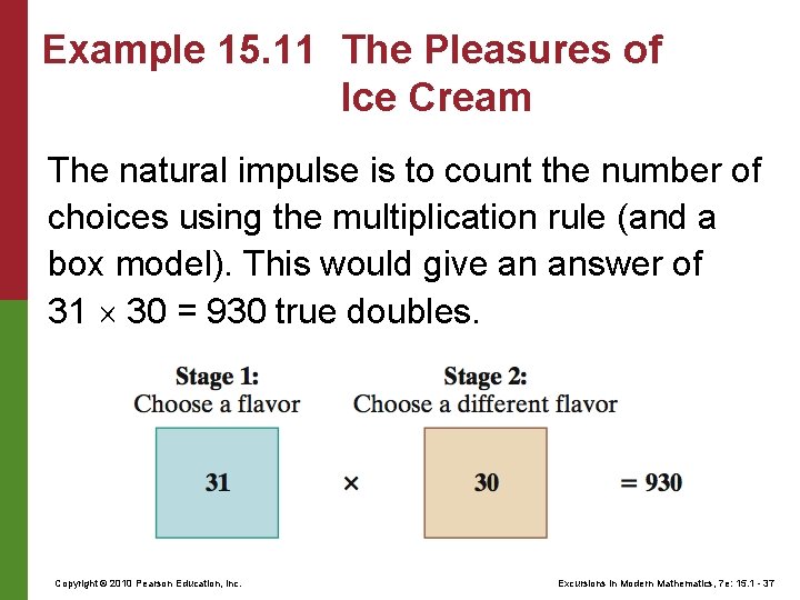
Example 15. 11 The Pleasures of Ice Cream The natural impulse is to count the number of choices using the multiplication rule (and a box model). This would give an answer of 31 30 = 930 true doubles. Copyright © 2010 Pearson Education, Inc. Excursions in Modern Mathematics, 7 e: 15. 1 - 37

Example 15. 11 The Pleasures of Ice Cream Unfortunately, this answer is double counting each of the true doubles. Why? When we use the multiplication rule, there is a well-defined order to things, and a scoop of strawberry followed by a scoop of chocolate is counted separately from a scoop of chocolate followed by a scoop of strawberry. But by all reasonable standards, a bowl of chocolatestrawberry is the same as a bowl of strawberry-chocolate. Copyright © 2010 Pearson Education, Inc. Excursions in Modern Mathematics, 7 e: 15. 1 - 38

Example 11 The Pleasures of Ice Cream The good news is that now that we understand why the count of 930 is wrong we can fix it. All we have to do to get the correct answer is to divide the original count by 2. It follows that the number of true double choices at Baskin-Robbins is (31/30)/2 = 465. Note: This is not necessarily true when the ice cream is served in a cone. Fussy people can be very picky about the order of the flavors when the scoops are stacked up. Copyright © 2010 Pearson Education, Inc. Excursions in Modern Mathematics, 7 e: 15. 1 - 39

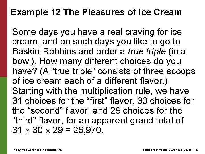
Example 12 The Pleasures of Ice Cream Some days you have a real craving for ice cream, and on such days you like to go to Baskin-Robbins and order a true triple (in a bowl). How many different choices do you have? (A “true triple” consists of three scoops of ice cream each of a different flavor. ) Starting with the multiplication rule, we have 31 choices for the “first” flavor, 30 choices for the “second” flavor, and 29 choices for the “third” flavor, for an apparent grand total of 31 30 29 = 26, 970. Copyright © 2010 Pearson Education, Inc. Excursions in Modern Mathematics, 7 e: 15. 1 - 40

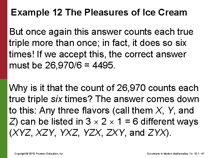
Example 12 The Pleasures of Ice Cream But once again this answer counts each true triple more than once; in fact, it does so six times! If we accept this, the correct answer must be 26, 970/6 = 4495. Why is it that the count of 26, 970 counts each true triple six times? The answer comes down to this: Any three flavors (call them X, Y, and Z) can be listed in 3 2 1 = 6 different ways (XYZ, XZY, YXZ, YZX, ZXY, and ZYX). Copyright © 2010 Pearson Education, Inc. Excursions in Modern Mathematics, 7 e: 15. 1 - 41

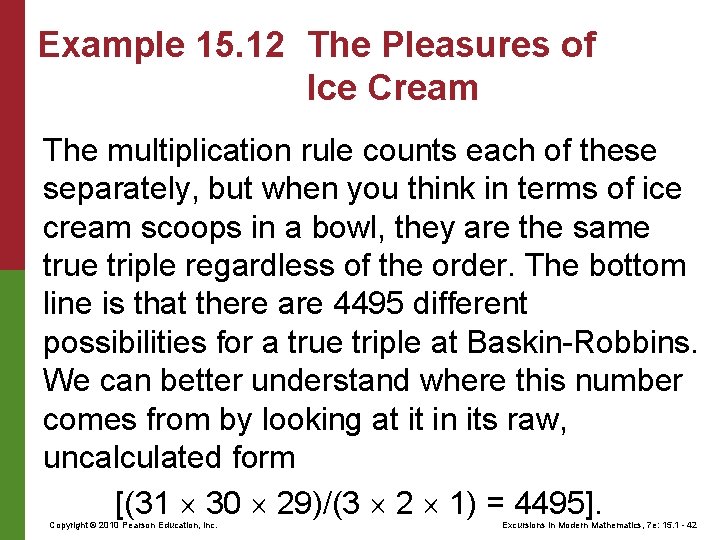
Example 15. 12 The Pleasures of Ice Cream The multiplication rule counts each of these separately, but when you think in terms of ice cream scoops in a bowl, they are the same true triple regardless of the order. The bottom line is that there are 4495 different possibilities for a true triple at Baskin-Robbins. We can better understand where this number comes from by looking at it in its raw, uncalculated form [(31 30 29)/(3 2 1) = 4495]. Copyright © 2010 Pearson Education, Inc. Excursions in Modern Mathematics, 7 e: 15. 1 - 42

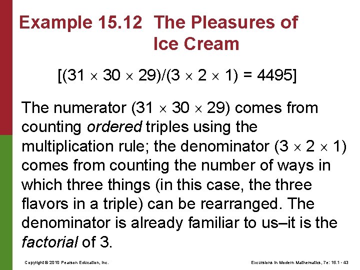
Example 15. 12 The Pleasures of Ice Cream [(31 30 29)/(3 2 1) = 4495] The numerator (31 30 29) comes from counting ordered triples using the multiplication rule; the denominator (3 2 1) comes from counting the number of ways in which three things (in this case, the three flavors in a triple) can be rearranged. The denominator is already familiar to us–it is the factorial of 3. Copyright © 2010 Pearson Education, Inc. Excursions in Modern Mathematics, 7 e: 15. 1 - 43

Example 15. 13 Five-Card Poker Hands We will compare two types of games: fivecard stud poker and five-card draw poker. In both of these games a player ends up with five cards, but there is an important difference when analyzing the mathematics behind the games: In five-card draw the order in which the cards come up is irrelevant; in five-card stud the order in which the cards come up is extremely relevant. Copyright © 2010 Pearson Education, Inc. Excursions in Modern Mathematics, 7 e: 15. 1 - 44

Example 15. 13 Five-Card Poker Hands The reason for this is that in five-card draw all cards are dealt down, but in five-card stud only the first card is dealt down–the remaining four cards are dealt up, one at a time. This means that players can assess the relative strengths of the other players’ hands as the game progresses and play their hands accordingly. Copyright © 2010 Pearson Education, Inc. Excursions in Modern Mathematics, 7 e: 15. 1 - 45

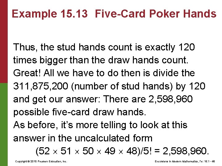
Example 15. 13 Five-Card Poker Hands Counting the number of five-card stud poker hands is a direct application of the multiplication rule: 52 possibilities for the first card, 51 for the second card, 50 for the third card, 49 for the fourth card, and 48 for the fifth card, for an awesome total of 52 51 50 49 48 = 311, 875, 200 possible hands. Copyright © 2010 Pearson Education, Inc. Excursions in Modern Mathematics, 7 e: 15. 1 - 46

Example 15. 13 Five-Card Poker Hands Counting the number of five-card draw poker hands requires a little more finesse. Here a player gets five down cards and the hand is the same regardless of the order in which the cards are dealt. There are 5! = 120 different ways in which the same set of five cards can be ordered, so that one draw hand corresponds to 120 different stud hands. Copyright © 2010 Pearson Education, Inc. Excursions in Modern Mathematics, 7 e: 15. 1 - 47

Example 15. 13 Five-Card Poker Hands Thus, the stud hands count is exactly 120 times bigger than the draw hands count. Great! All we have to do then is divide the 311, 875, 200 (number of stud hands) by 120 and get our answer: There are 2, 598, 960 possible five-card draw hands. As before, it’s more telling to look at this answer in the uncalculated form (52 51 50 49 48)/5! = 2, 598, 960. Copyright © 2010 Pearson Education, Inc. Excursions in Modern Mathematics, 7 e: 15. 1 - 48

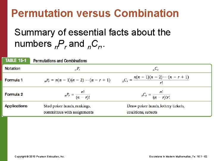
Permutation versus Combination Suppose that we have a set of n distinct objects and we want to select r different objects from this set. The number of ways that this can be done depends on whether the selections are ordered or unordered. Ordered selections are the generalization of stud poker hands–selecting the same objects in different order gets you something different. Copyright © 2010 Pearson Education, Inc. Excursions in Modern Mathematics, 7 e: 15. 1 - 49

Permutation versus Combination Unordered selections are the generalization of draw poker hands–selecting the same objects in different order gets you nothing new. To distinguish between these two scenarios, we use the terms permutation to describe an ordered selection and combination to describe an unordered selection. Copyright © 2010 Pearson Education, Inc. Excursions in Modern Mathematics, 7 e: 15. 1 - 50

Permutation versus Combination For a given number of objects n and a given selection size r (where 0 ≤ r ≤ n) we can talk about the “number of permutations of n objects taken r at a time” and the “number of combinations of n objects taken r at a time, ” and these two extremely important families of numbers are denoted n. Pr and n. Cr, respectively. (Some calculators use variations of this notation, such as Pn, r and Cn, r respectively. ) Copyright © 2010 Pearson Education, Inc. Excursions in Modern Mathematics, 7 e: 15. 1 - 51

Permutation versus Combination Summary of essential facts about the numbers n. Pr and n. Cr, . Copyright © 2010 Pearson Education, Inc. Excursions in Modern Mathematics, 7 e: 15. 1 - 52

Example 15. 14 The Florida Lotto Like many other state lotteries, the Florida Lotto is a game in which for a small investment of just one dollar a player has a chance of winning tens of millions of dollars. Enormous upside, hardly any downside–that’s why people love playing the lottery and, like they say, “everybody has to have a dream. ” But, in general, lotteries are a very bad investment, even if it’s only a dollar, and the dreams can turn to nightmares. Why so? Copyright © 2010 Pearson Education, Inc. Excursions in Modern Mathematics, 7 e: 15. 1 - 53

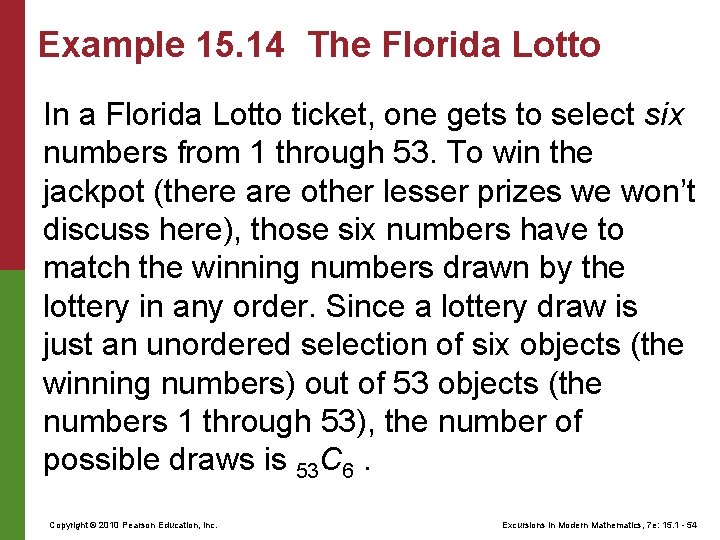
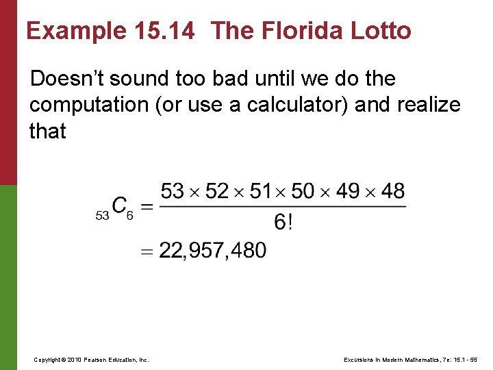
Example 15. 14 The Florida Lotto In a Florida Lotto ticket, one gets to select six numbers from 1 through 53. To win the jackpot (there are other lesser prizes we won’t discuss here), those six numbers have to match the winning numbers drawn by the lottery in any order. Since a lottery draw is just an unordered selection of six objects (the winning numbers) out of 53 objects (the numbers 1 through 53), the number of possible draws is 53 C 6. Copyright © 2010 Pearson Education, Inc. Excursions in Modern Mathematics, 7 e: 15. 1 - 54

Example 15. 14 The Florida Lotto Doesn’t sound too bad until we do the computation (or use a calculator) and realize that Copyright © 2010 Pearson Education, Inc. Excursions in Modern Mathematics, 7 e: 15. 1 - 55

Chapter 15 - 4 15. 1 Random Experiments and Sample Spaces 15. 2 Counting Outcomes in Sample Spaces 15. 3 Permutations and Combinations 15. 4 Probability Spaces 15. 5 Equiprobable Spaces 15. 6 Odds Copyright © 2010 Pearson Education, Inc. Excursions in Modern Mathematics, 7 e: 15. 1 - 56

What is Probability? If we toss a coin in the air, what is the probability that it will land heads up? This one is not a very profound question, and almost everybody agrees on the answer, although not necessarily for the same reason. The standard answer given is 1 out of 2, or 1/2. But why is the answer 1/2 and what does such an answer mean? Copyright © 2010 Pearson Education, Inc. Excursions in Modern Mathematics, 7 e: 15. 1 - 57

What is Probability? One common explanation given for the answer of 1/2 is that when we toss a coin, there are two possible outcomes (H and T), and since H represents one of the two possibilities, the probability of the outcome H must be 1 out of 2 or 1/2. This logic, while correct in the case of an honest coin, has a lot of holes in it. Copyright © 2010 Pearson Education, Inc. Excursions in Modern Mathematics, 7 e: 15. 1 - 58

Example 15. 15 Who Is Shooting Those Free Throws? Imagine an NBA player in the act of shooting a free throw. Just like with a coin toss, there are two possible outcomes to the free-throw shot (success or failure), but it would be absurd to conclude that the probability of making the free throw is therefore 1 out of 2, or 1/2. Here the two outcomes are not both equally likely, and their probabilities should reflect that. Copyright © 2010 Pearson Education, Inc. Excursions in Modern Mathematics, 7 e: 15. 1 - 59

Example 15. 15 Who Is Shooting Those Free Throws? The probability of a basketball player making a free throw very much depends on the abilities of the player doing the shooting–it makes a difference if it’s Steve Nash or Shaquille O’Neal. Nash is one of the best free -throw shooters in the history of the NBA, with a career average of 90%, while Shaq is a notoriously poor free-throw shooter (52% career average). Copyright © 2010 Pearson Education, Inc. Excursions in Modern Mathematics, 7 e: 15. 1 - 60

Empirical Interpretation of Probability Example 15. 15 leads us to what is known as the empirical interpretation of the concept of probability. Under this interpretation when tossing an honest coin the probability of Heads is 1/2 not because Heads is one out of two possible outcomes but because, if we were to toss the coin over and over– hundreds, possibly thousands, of times–in the long run about half of the tosses will turn out to be heads, a fact that has been confirmed by experiment many times. Copyright © 2010 Pearson Education, Inc. Excursions in Modern Mathematics, 7 e: 15. 1 - 61

Probability Theory The argument as to exactly how to interpret the statement “the probability of X is such and such” goes back to the late 1600 s, and it wasn’t until the 1930 s that a formal theory for dealing with probabilities was developed by the Russian mathematician A. N. Kolmogorov (1903– 1987). This theory has made probability one of the most useful and important concepts in modern mathematics. In the remainder of this chapter we will discuss some of the basic concepts of probability theory. Copyright © 2010 Pearson Education, Inc. Excursions in Modern Mathematics, 7 e: 15. 1 - 62

Events An event is any subset of the sample space. That is, an event is any set of individual outcomes. (This definition includes the possibility of an “event” that has no outcomes as well as events consisting of a single outcome. ) By definition, events are sets (subsets of the sample space), and we will deal with events using set notation as well as the basic rules of set theory. Copyright © 2010 Pearson Education, Inc. Excursions in Modern Mathematics, 7 e: 15. 1 - 63

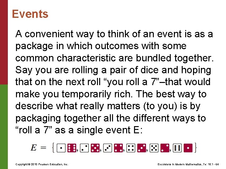
Events A convenient way to think of an event is as a package in which outcomes with some common characteristic are bundled together. Say you are rolling a pair of dice and hoping that on the next roll “you roll a 7”–that would make you temporarily rich. The best way to describe what really matters (to you) is by packaging together all the different ways to “roll a 7” as a single event E: Copyright © 2010 Pearson Education, Inc. Excursions in Modern Mathematics, 7 e: 15. 1 - 64

Events Sometimes an event consists of just one outcome. We will call such an event a simple event. In some sense simple events are the building blocks for all other events (more on that later). There is also the special case of the empty set { }, corresponding to an event with no outcomes. Such an event can never happen, and thus we call it the impossible event. Copyright © 2010 Pearson Education, Inc. Excursions in Modern Mathematics, 7 e: 15. 1 - 65

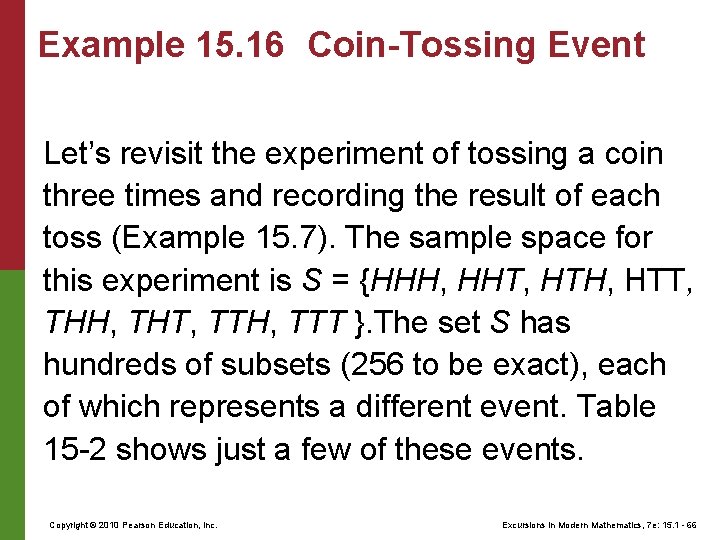
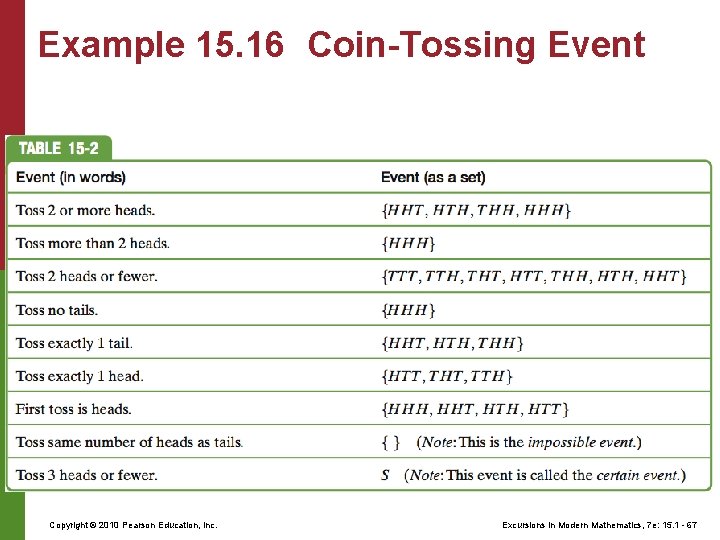
Example 15. 16 Coin-Tossing Event Let’s revisit the experiment of tossing a coin three times and recording the result of each toss (Example 15. 7). The sample space for this experiment is S = {HHH, HHT, HTH, HTT, THH, THT, TTH, TTT }. The set S has hundreds of subsets (256 to be exact), each of which represents a different event. Table 15 -2 shows just a few of these events. Copyright © 2010 Pearson Education, Inc. Excursions in Modern Mathematics, 7 e: 15. 1 - 66

Example 15. 16 Coin-Tossing Event Copyright © 2010 Pearson Education, Inc. Excursions in Modern Mathematics, 7 e: 15. 1 - 67

Example 15. 17 The Unknown Free-Throw Shooter A player is going to shoot a free throw. We know nothing about his or her abilities–for all we know, the player could be Steve Nash, or Shaquille O’Neal, or Joe Schmoe, or you, or me. How can we describe the probability that he or she will make that free throw? It seems that there is no way to answer this question, since we know nothing about the ability of the shooter. We could argue that the probability could be just about any number between 0 and 1. Copyright © 2010 Pearson Education, Inc. Excursions in Modern Mathematics, 7 e: 15. 1 - 68

Example 15. 17 The Unknown Free-Throw Shooter No problem–we make our unknown probability a variable, say p. What can we say about the probability that our shooter misses the free throw? A lot. Since there are only two possible outcomes in the sample space S = {s, f } the probability of success (s) and the probability of failure (f) must complement each other–in other words, must add up to 1. This means that the probability of missing the free throw must be 1 – p. Copyright © 2010 Pearson Education, Inc. Excursions in Modern Mathematics, 7 e: 15. 1 - 69

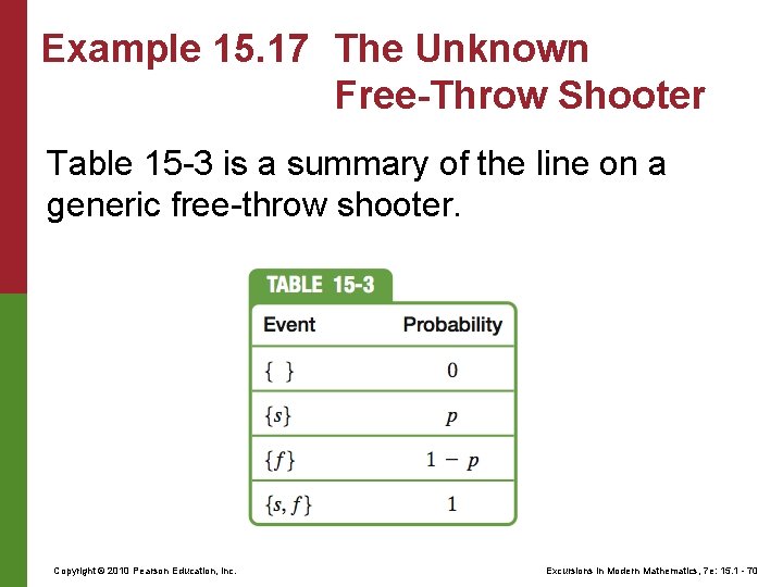
Example 15. 17 The Unknown Free-Throw Shooter Table 15 -3 is a summary of the line on a generic free-throw shooter. Copyright © 2010 Pearson Education, Inc. Excursions in Modern Mathematics, 7 e: 15. 1 - 70

Example 15. 17 The Unknown Free-Throw Shooter Humble as it may seem, Table 15 -3 gives a complete model of free-throw shooting. It works when the free-throw shooter is Steve Nash (make it p = 0. 90 ), Shaquille O’Neal (make it p = 0. 52), or the author of this book (make it p = 0. 30). Each one of the choices results in a different assignment of numbers to the outcomes in the sample space. Copyright © 2010 Pearson Education, Inc. Excursions in Modern Mathematics, 7 e: 15. 1 - 71

Probability Assignment Example 15. 17 illustrates the concept of a probability assignment. A probability assignment is a function that assigns to each event E a number between 0 and 1, which represents the probability of the event E and which we denote by Pr(E). A probability assignment always assigns probability 0 to the impossible event [Pr({ }) = 0 and probability 1 to the whole sample space [Pr(S) = 1]. Copyright © 2010 Pearson Education, Inc. Excursions in Modern Mathematics, 7 e: 15. 1 - 72

Probability Assignment With finite sample spaces a probability assignment is defined by assigning probabilities to just the simple events in the sample space. Once we do this, we can find the probability of any event by simply adding the probabilities of the individual outcomes that make up that event. There are only two requirements for a valid probability assignment: (1) All probabilities are numbers between 0 and 1, and (2) the sum of the probabilities of the simple events equals 1. Copyright © 2010 Pearson Education, Inc. Excursions in Modern Mathematics, 7 e: 15. 1 - 73

Example 15. 18 Handicapping a Tennis Tournament There are six players playing in a tennis tournament: A (Russian, female), B (Croatian, male), C (Australian, male), D (Swiss, male), E (American, female), and F (American, female). To handicap the winner of the tournament we need a probability assignment on the sample space S = {A, B, C, D, E, F }. Copyright © 2010 Pearson Education, Inc. Excursions in Modern Mathematics, 7 e: 15. 1 - 74

Example 15. 18 Handicapping a Tennis Tournament With sporting events the probability assignment is subjective (it reflects an opinion), but professional odds-makers are usually very good at getting close to the right probabilities. For example, imagine that a professional odds-maker comes up with the following probability assignment: Pr(A) = 0. 08, Pr(B) = 0. 16, Pr(C) = 0. 20, Pr(D) = 0. 25, Pr(E) = 0. 16, Pr(F) = 0. 15. Copyright © 2010 Pearson Education, Inc. Excursions in Modern Mathematics, 7 e: 15. 1 - 75

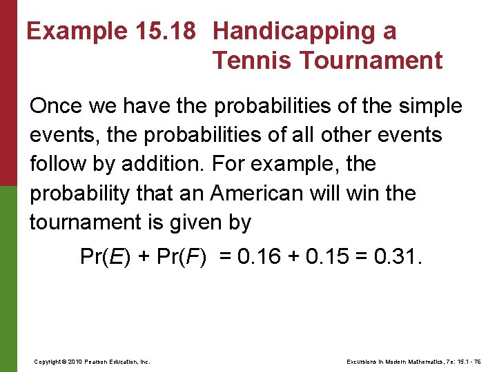
Example 15. 18 Handicapping a Tennis Tournament Once we have the probabilities of the simple events, the probabilities of all other events follow by addition. For example, the probability that an American will win the tournament is given by Pr(E) + Pr(F) = 0. 16 + 0. 15 = 0. 31. Copyright © 2010 Pearson Education, Inc. Excursions in Modern Mathematics, 7 e: 15. 1 - 76

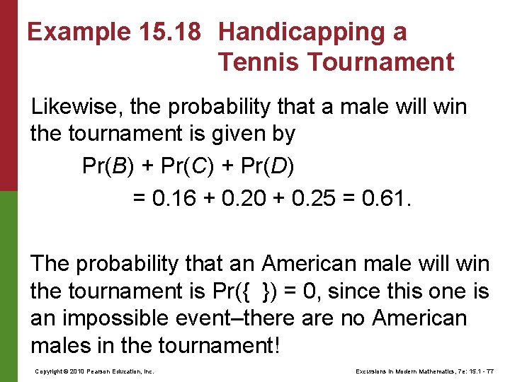
Example 15. 18 Handicapping a Tennis Tournament Likewise, the probability that a male will win the tournament is given by Pr(B) + Pr(C) + Pr(D) = 0. 16 + 0. 20 + 0. 25 = 0. 61. The probability that an American male will win the tournament is Pr({ }) = 0, since this one is an impossible event–there are no American males in the tournament! Copyright © 2010 Pearson Education, Inc. Excursions in Modern Mathematics, 7 e: 15. 1 - 77

Probability Space Once a specific probability assignment is made on a sample space, the combination of the sample space and the probability assignment is called a probability space. The following is a summary of the key facts related to probability spaces. Copyright © 2010 Pearson Education, Inc. Excursions in Modern Mathematics, 7 e: 15. 1 - 78

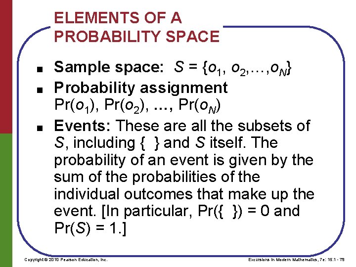
ELEMENTS OF A PROBABILITY SPACE ■ ■ ■ Sample space: S = {o 1, o 2, …, o. N} Probability assignment Pr(o 1), Pr(o 2), …, Pr(o. N) Events: These are all the subsets of S, including { } and S itself. The probability of an event is given by the sum of the probabilities of the individual outcomes that make up the event. [In particular, Pr({ }) = 0 and Pr(S) = 1. ] Copyright © 2010 Pearson Education, Inc. Excursions in Modern Mathematics, 7 e: 15. 1 - 79

Chapter 15 - 5 15. 1 Random Experiments and Sample Spaces 15. 2 Counting Outcomes in Sample Spaces 15. 3 Permutations and Combinations 15. 4 Probability Spaces 15. 5 Equiprobable Spaces 15. 6 Odds Copyright © 2010 Pearson Education, Inc. Excursions in Modern Mathematics, 7 e: 15. 1 - 80

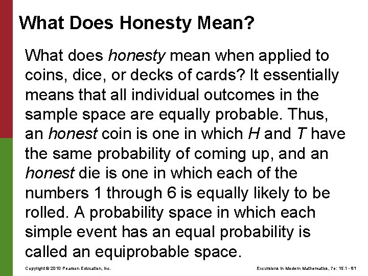
What Does Honesty Mean? What does honesty mean when applied to coins, dice, or decks of cards? It essentially means that all individual outcomes in the sample space are equally probable. Thus, an honest coin is one in which H and T have the same probability of coming up, and an honest die is one in which each of the numbers 1 through 6 is equally likely to be rolled. A probability space in which each simple event has an equal probability is called an equiprobable space. Copyright © 2010 Pearson Education, Inc. Excursions in Modern Mathematics, 7 e: 15. 1 - 81

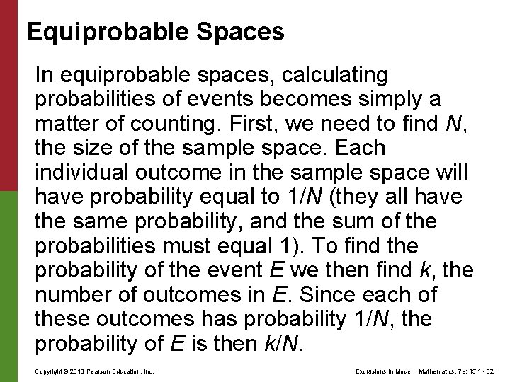
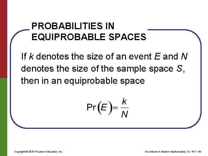
Equiprobable Spaces In equiprobable spaces, calculating probabilities of events becomes simply a matter of counting. First, we need to find N, the size of the sample space. Each individual outcome in the sample space will have probability equal to 1/N (they all have the same probability, and the sum of the probabilities must equal 1). To find the probability of the event E we then find k, the number of outcomes in E. Since each of these outcomes has probability 1/N, the probability of E is then k/N. Copyright © 2010 Pearson Education, Inc. Excursions in Modern Mathematics, 7 e: 15. 1 - 82

PROBABILITIES IN EQUIPROBABLE SPACES If k denotes the size of an event E and N denotes the size of the sample space S, then in an equiprobable space Copyright © 2010 Pearson Education, Inc. Excursions in Modern Mathematics, 7 e: 15. 1 - 83

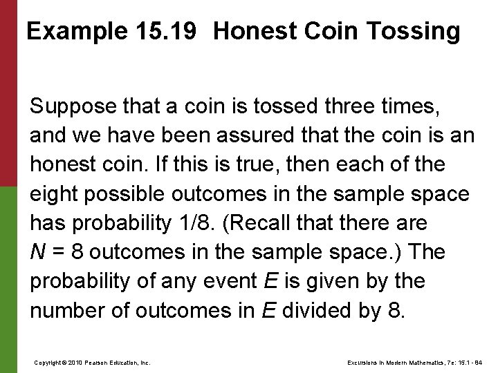
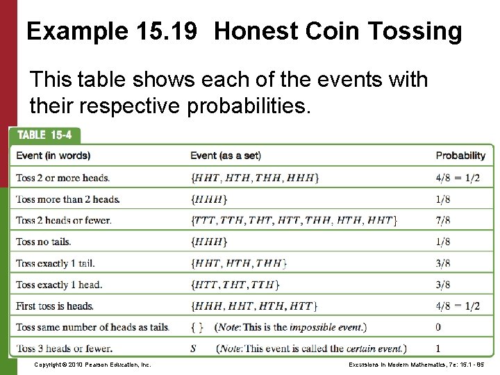
Example 15. 19 Honest Coin Tossing Suppose that a coin is tossed three times, and we have been assured that the coin is an honest coin. If this is true, then each of the eight possible outcomes in the sample space has probability 1/8. (Recall that there are N = 8 outcomes in the sample space. ) The probability of any event E is given by the number of outcomes in E divided by 8. Copyright © 2010 Pearson Education, Inc. Excursions in Modern Mathematics, 7 e: 15. 1 - 84

Example 15. 19 Honest Coin Tossing This table shows each of the events with their respective probabilities. Copyright © 2010 Pearson Education, Inc. Excursions in Modern Mathematics, 7 e: 15. 1 - 85

Example 15. 20 Rolling a Pair of Honest Dice Imagine that you are playing some game that involves rolling a pair of honest dice, and the only thing that matters is the total of the two numbers rolled. As we saw in Example 15. 4 the sample space in this situation is S = {2, 3, 4, 5, 6, 7, 8, 9, 10, 11, 12}, where the outcomes are the possible totals that could be rolled. Copyright © 2010 Pearson Education, Inc. Excursions in Modern Mathematics, 7 e: 15. 1 - 86

Example 15. 20 Rolling a Pair of Honest Dice This sample space has N = 11 possible outcomes, but the outcomes are not equally likely, so it would be wrong to assign to each outcome the probability 1/11. In fact, most people with some experience rolling a pair of dice know that the likelihood of rolling a 7 is much higher than that of rolling a 12. Copyright © 2010 Pearson Education, Inc. Excursions in Modern Mathematics, 7 e: 15. 1 - 87

Example 15. 20 Rolling a Pair of Honest Dice How can we find the exact probabilities for the various totals that one might roll? We can answer this question by considering the sample space discussed in Example 15. 5, where every one of the N = 36 possible rolls is listed as a separate outcome. Because the dice are honest, each of these 36 possible outcomes is equally likely to occur, so the probability of each is 1/36. Now we have something! Copyright © 2010 Pearson Education, Inc. Excursions in Modern Mathematics, 7 e: 15. 1 - 88

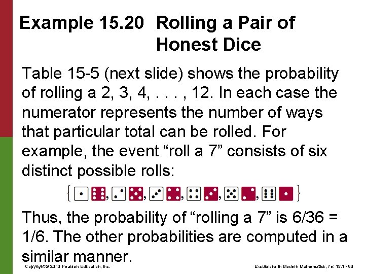
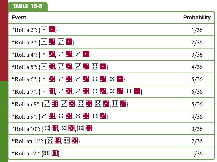
Example 15. 20 Rolling a Pair of Honest Dice Table 15 -5 (next slide) shows the probability of rolling a 2, 3, 4, . . . , 12. In each case the numerator represents the number of ways that particular total can be rolled. For example, the event “roll a 7” consists of six distinct possible rolls: Thus, the probability of “rolling a 7” is 6/36 = 1/6. The other probabilities are computed in a similar manner. Copyright © 2010 Pearson Education, Inc. Excursions in Modern Mathematics, 7 e: 15. 1 - 89

Copyright © 2010 Pearson Education, Inc. Excursions in Modern Mathematics, 7 e: 15. 1 - 90

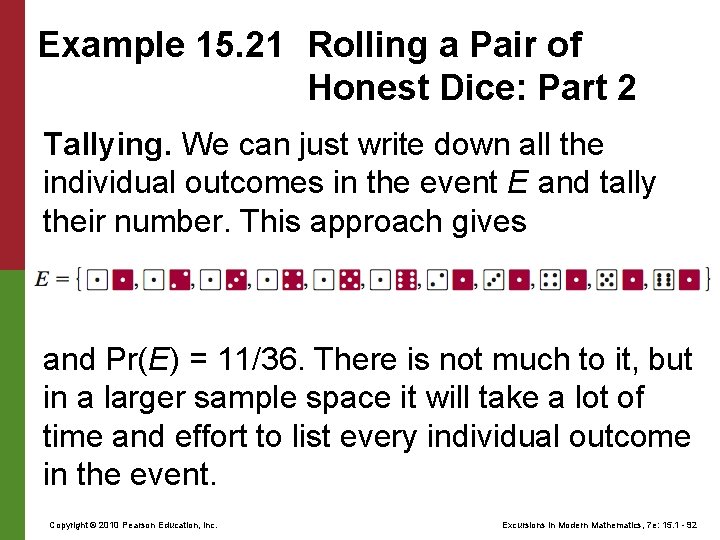
Example 15. 21 Rolling a Pair of Honest Dice: Part 2 Once again, we are rolling a pair of honest dice. We are now going to find the probability of the event E: “at least one of the dice comes up an ace. ”(In dice jargon, a is called an ace. ) This is a slightly more sophisticated counting question than the ones in Example 15. 20. We will show three different ways to answer the question. Copyright © 2010 Pearson Education, Inc. Excursions in Modern Mathematics, 7 e: 15. 1 - 91

Example 15. 21 Rolling a Pair of Honest Dice: Part 2 Tallying. We can just write down all the individual outcomes in the event E and tally their number. This approach gives and Pr(E) = 11/36. There is not much to it, but in a larger sample space it will take a lot of time and effort to list every individual outcome in the event. Copyright © 2010 Pearson Education, Inc. Excursions in Modern Mathematics, 7 e: 15. 1 - 92

Example 15. 21 Rolling a Pair of Honest Dice: Part 2 Complementary Event. Behind this approach is the germ of a really important idea. Imagine that you are playing a game, and you win if at least one of the two numbers comes up an ace (that’s event E). Otherwise you lose (call that event F). The two events E and F are called complementary events, and E is called the complement of F(and vice versa). Copyright © 2010 Pearson Education, Inc. Excursions in Modern Mathematics, 7 e: 15. 1 - 93

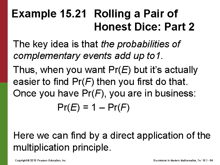
Example 15. 21 Rolling a Pair of Honest Dice: Part 2 The key idea is that the probabilities of complementary events add up to 1. Thus, when you want Pr(E) but it’s actually easier to find Pr(F) then you first do that. Once you have Pr(F), you are in business: Pr(E) = 1 – Pr(F) Here we can find by a direct application of the multiplication principle. Copyright © 2010 Pearson Education, Inc. Excursions in Modern Mathematics, 7 e: 15. 1 - 94

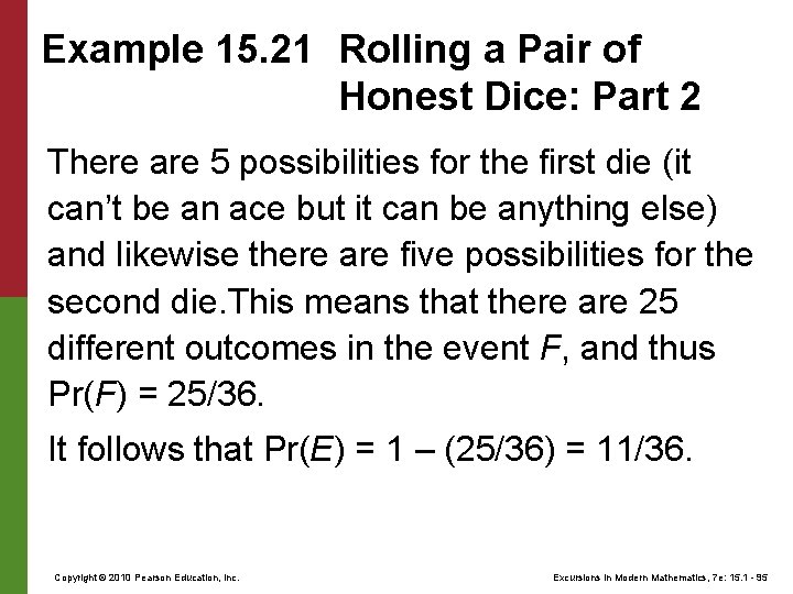
Example 15. 21 Rolling a Pair of Honest Dice: Part 2 There are 5 possibilities for the first die (it can’t be an ace but it can be anything else) and likewise there are five possibilities for the second die. This means that there are 25 different outcomes in the event F, and thus Pr(F) = 25/36. It follows that Pr(E) = 1 – (25/36) = 11/36. Copyright © 2010 Pearson Education, Inc. Excursions in Modern Mathematics, 7 e: 15. 1 - 95

Example 15. 21 Rolling a Pair of Honest Dice: Part 2 Independent Events. In this approach, we look at each die separately and, as usual, pretend that one die is white and the other one is red. We will let F 1 denote the event “the white die does not come up an ace” and F 2 denote the event “the red die does not come up an ace. ” Copyright © 2010 Pearson Education, Inc. Excursions in Modern Mathematics, 7 e: 15. 1 - 96

Example 15. 21 Rolling a Pair of Honest Dice: Part 2 Clearly, Pr(F 1) = 5/6 and Pr(F 2) = 5/6 and Now comes a critical observation: The probability that both events F 1 and F 2 happen can be found by multiplying their respective probabilities. This means that Pr(F) = (5/6) = 25/36. We can now find Pr(E) exactly as before: Pr(E) = 1 – Pr(F) = 1 – (25/36) = 11/36. Copyright © 2010 Pearson Education, Inc. Excursions in Modern Mathematics, 7 e: 15. 1 - 97

Independent Events Of the three approaches used in Example 15. 20, the last approach appears to be the most convoluted, but, in fact, it is the one with the most promise. It is based on the concept of independence of events. Two events are said to be independent events if the occurrence of one event does not affect the probability of the occurrence of the other. Copyright © 2010 Pearson Education, Inc. Excursions in Modern Mathematics, 7 e: 15. 1 - 98

Independent Events When events E and F are independent, the probability that both occur is the product of their respective probabilities; in other words, Pr(E and F) = Pr(E) • Pr(F). This is called the multiplication principle for independent events. Copyright © 2010 Pearson Education, Inc. Excursions in Modern Mathematics, 7 e: 15. 1 - 99

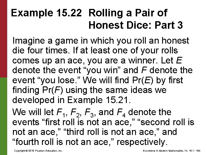
Example 15. 22 Rolling a Pair of Honest Dice: Part 3 Imagine a game in which you roll an honest die four times. If at least one of your rolls comes up an ace, you are a winner. Let E denote the event “you win” and F denote the event “you lose. ” We will find Pr(E) by first finding Pr(F) using the same ideas we developed in Example 15. 21. We will let F 1, F 2, F 3, and F 4 denote the events “first roll is not an ace, ” “second roll is not an ace, ” “third roll is not an ace, ” and “fourth roll is not an ace, ” respectively. Copyright © 2010 Pearson Education, Inc. Excursions in Modern Mathematics, 7 e: 15. 1 - 100

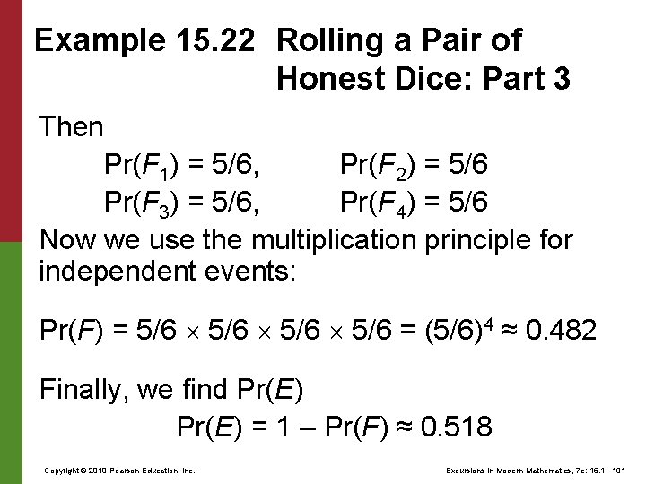
Example 15. 22 Rolling a Pair of Honest Dice: Part 3 Then Pr(F 1) = 5/6, Pr(F 2) = 5/6 Pr(F 3) = 5/6, Pr(F 4) = 5/6 Now we use the multiplication principle for independent events: Pr(F) = 5/6 = (5/6)4 ≈ 0. 482 Finally, we find Pr(E) = 1 – Pr(F) ≈ 0. 518 Copyright © 2010 Pearson Education, Inc. Excursions in Modern Mathematics, 7 e: 15. 1 - 101

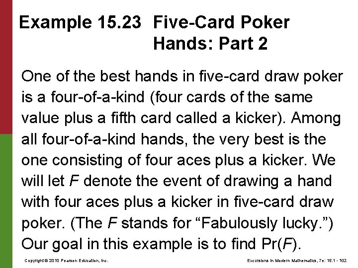
Example 15. 23 Five-Card Poker Hands: Part 2 One of the best hands in five-card draw poker is a four-of-a-kind (four cards of the same value plus a fifth card called a kicker). Among all four-of-a-kind hands, the very best is the one consisting of four aces plus a kicker. We will let F denote the event of drawing a hand with four aces plus a kicker in five-card draw poker. (The F stands for “Fabulously lucky. ”) Our goal in this example is to find Pr(F). Copyright © 2010 Pearson Education, Inc. Excursions in Modern Mathematics, 7 e: 15. 1 - 102

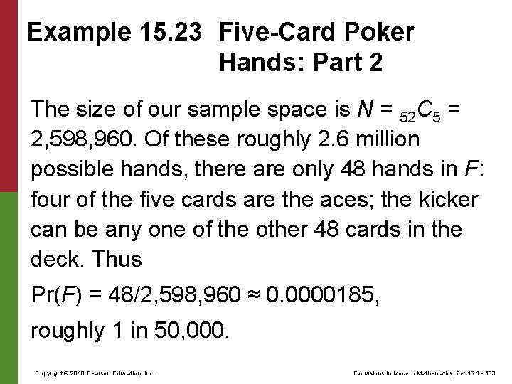
Example 15. 23 Five-Card Poker Hands: Part 2 The size of our sample space is N = 52 C 5 = 2, 598, 960. Of these roughly 2. 6 million possible hands, there are only 48 hands in F: four of the five cards are the aces; the kicker can be any one of the other 48 cards in the deck. Thus Pr(F) = 48/2, 598, 960 ≈ 0. 0000185, roughly 1 in 50, 000. Copyright © 2010 Pearson Education, Inc. Excursions in Modern Mathematics, 7 e: 15. 1 - 103

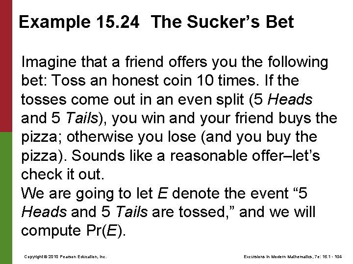
Example 15. 24 The Sucker’s Bet Imagine that a friend offers you the following bet: Toss an honest coin 10 times. If the tosses come out in an even split (5 Heads and 5 Tails), you win and your friend buys the pizza; otherwise you lose (and you buy the pizza). Sounds like a reasonable offer–let’s check it out. We are going to let E denote the event “ 5 Heads and 5 Tails are tossed, ” and we will compute Pr(E). Copyright © 2010 Pearson Education, Inc. Excursions in Modern Mathematics, 7 e: 15. 1 - 104

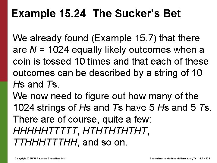
Example 15. 24 The Sucker’s Bet We already found (Example 15. 7) that there are N = 1024 equally likely outcomes when a coin is tossed 10 times and that each of these outcomes can be described by a string of 10 Hs and Ts. We now need to figure out how many of the 1024 strings of Hs and Ts have 5 Hs and 5 Ts. There are of course, quite a few: HHHHHTTTTT, HTHTHT, TTHHHTTTHH, and so on. Copyright © 2010 Pearson Education, Inc. Excursions in Modern Mathematics, 7 e: 15. 1 - 105

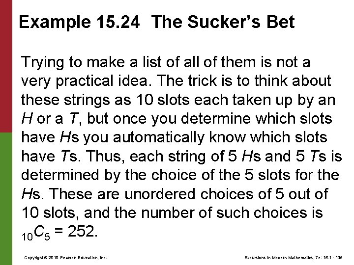
Example 15. 24 The Sucker’s Bet Trying to make a list of all of them is not a very practical idea. The trick is to think about these strings as 10 slots each taken up by an H or a T, but once you determine which slots have Hs you automatically know which slots have Ts. Thus, each string of 5 Hs and 5 Ts is determined by the choice of the 5 slots for the Hs. These are unordered choices of 5 out of 10 slots, and the number of such choices is 10 C 5 = 252. Copyright © 2010 Pearson Education, Inc. Excursions in Modern Mathematics, 7 e: 15. 1 - 106

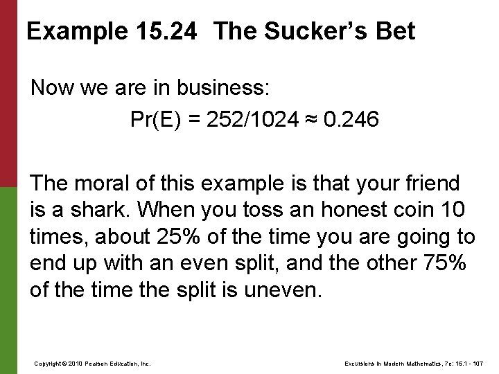
Example 15. 24 The Sucker’s Bet Now we are in business: Pr(E) = 252/1024 ≈ 0. 246 The moral of this example is that your friend is a shark. When you toss an honest coin 10 times, about 25% of the time you are going to end up with an even split, and the other 75% of the time the split is uneven. Copyright © 2010 Pearson Education, Inc. Excursions in Modern Mathematics, 7 e: 15. 1 - 107

Chapter 15 - 6 15. 1 Random Experiments and Sample Spaces 15. 2 Counting Outcomes in Sample Spaces 15. 3 Permutations and Combinations 15. 4 Probability Spaces 15. 5 Equiprobable Spaces 15. 6 Odds Copyright © 2010 Pearson Education, Inc. Excursions in Modern Mathematics, 7 e: 15. 1 - 108

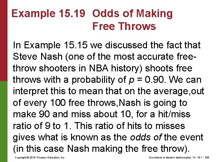
Example 15. 19 Odds of Making Free Throws In Example 15. 15 we discussed the fact that Steve Nash (one of the most accurate freethrow shooters in NBA history) shoots free throws with a probability of p = 0. 90. We can interpret this to mean that on the average, out of every 100 free throws, Nash is going to make 90 and miss about 10, for a hit/miss ratio of 9 to 1. This ratio of hits to misses gives what is known as the odds of the event (in this case Nash making the free throw). Copyright © 2010 Pearson Education, Inc. Excursions in Modern Mathematics, 7 e: 15. 1 - 109

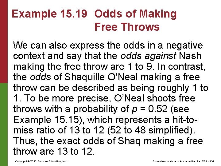
Example 15. 19 Odds of Making Free Throws We can also express the odds in a negative context and say that the odds against Nash making the free throw are 1 to 9. In contrast, the odds of Shaquille O’Neal making a free throw can be described as being roughly 1 to 1. To be more precise, O’Neal shoots free throws with a probability of p = 0. 52 (see Example 15. 15), which represents a hit-tomiss ratio of 13 to 12 (52 to 48 simplified). Thus, the exact odds of Shaq making a free throw are 13 to 12. Copyright © 2010 Pearson Education, Inc. Excursions in Modern Mathematics, 7 e: 15. 1 - 110

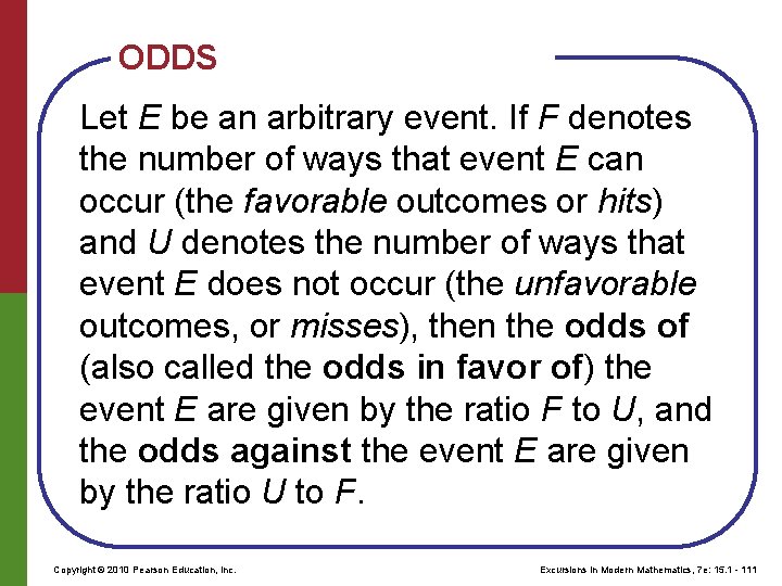
ODDS Let E be an arbitrary event. If F denotes the number of ways that event E can occur (the favorable outcomes or hits) and U denotes the number of ways that event E does not occur (the unfavorable outcomes, or misses), then the odds of (also called the odds in favor of) the event E are given by the ratio F to U, and the odds against the event E are given by the ratio U to F. Copyright © 2010 Pearson Education, Inc. Excursions in Modern Mathematics, 7 e: 15. 1 - 111

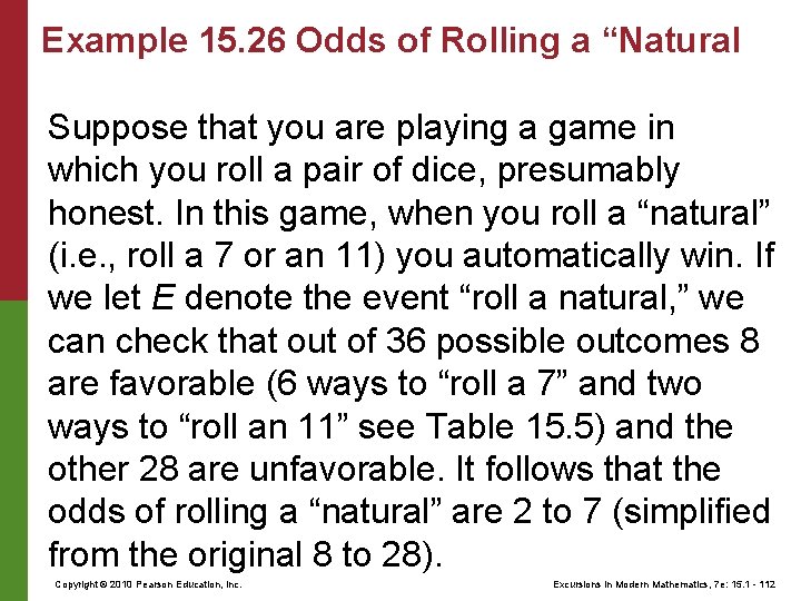
Example 15. 26 Odds of Rolling a “Natural Suppose that you are playing a game in which you roll a pair of dice, presumably honest. In this game, when you roll a “natural” (i. e. , roll a 7 or an 11) you automatically win. If we let E denote the event “roll a natural, ” we can check that out of 36 possible outcomes 8 are favorable (6 ways to “roll a 7” and two ways to “roll an 11” see Table 15. 5) and the other 28 are unfavorable. It follows that the odds of rolling a “natural” are 2 to 7 (simplified from the original 8 to 28). Copyright © 2010 Pearson Education, Inc. Excursions in Modern Mathematics, 7 e: 15. 1 - 112

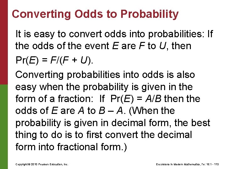
Converting Odds to Probability It is easy to convert odds into probabilities: If the odds of the event E are F to U, then Pr(E) = F/(F + U). Converting probabilities into odds is also easy when the probability is given in the form of a fraction: If Pr(E) = A/B then the odds of E are A to B – A. (When the probability is given in decimal form, the best thing to do is to first convert the decimal form into fractional form. ) Copyright © 2010 Pearson Education, Inc. Excursions in Modern Mathematics, 7 e: 15. 1 - 113

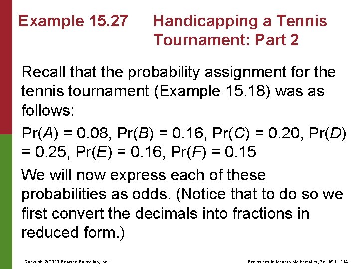
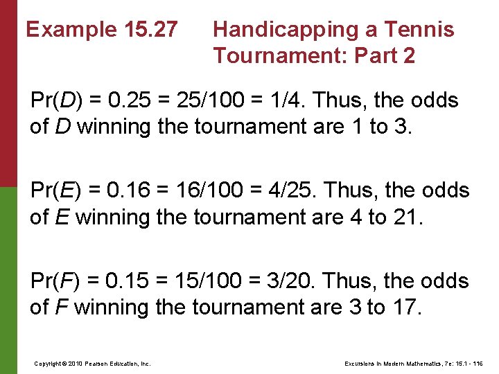
Example 15. 27 Handicapping a Tennis Tournament: Part 2 Recall that the probability assignment for the tennis tournament (Example 15. 18) was as follows: Pr(A) = 0. 08, Pr(B) = 0. 16, Pr(C) = 0. 20, Pr(D) = 0. 25, Pr(E) = 0. 16, Pr(F) = 0. 15 We will now express each of these probabilities as odds. (Notice that to do so we first convert the decimals into fractions in reduced form. ) Copyright © 2010 Pearson Education, Inc. Excursions in Modern Mathematics, 7 e: 15. 1 - 114

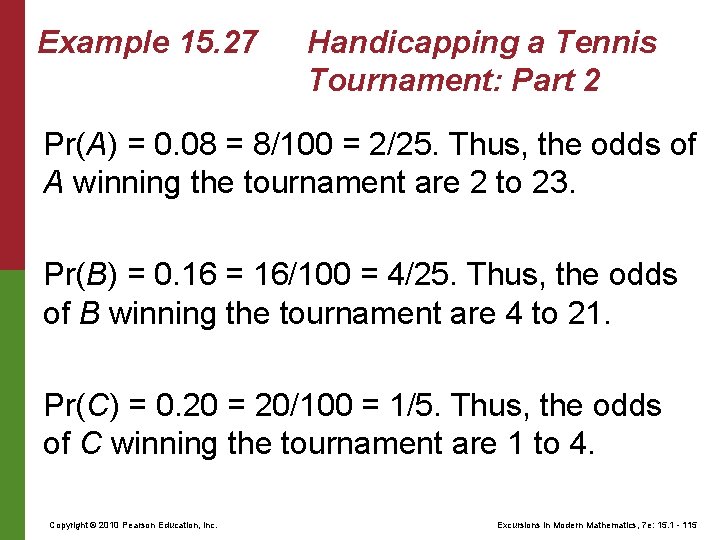
Example 15. 27 Handicapping a Tennis Tournament: Part 2 Pr(A) = 0. 08 = 8/100 = 2/25. Thus, the odds of A winning the tournament are 2 to 23. Pr(B) = 0. 16 = 16/100 = 4/25. Thus, the odds of B winning the tournament are 4 to 21. Pr(C) = 0. 20 = 20/100 = 1/5. Thus, the odds of C winning the tournament are 1 to 4. Copyright © 2010 Pearson Education, Inc. Excursions in Modern Mathematics, 7 e: 15. 1 - 115

Example 15. 27 Handicapping a Tennis Tournament: Part 2 Pr(D) = 0. 25 = 25/100 = 1/4. Thus, the odds of D winning the tournament are 1 to 3. Pr(E) = 0. 16 = 16/100 = 4/25. Thus, the odds of E winning the tournament are 4 to 21. Pr(F) = 0. 15 = 15/100 = 3/20. Thus, the odds of F winning the tournament are 3 to 17. Copyright © 2010 Pearson Education, Inc. Excursions in Modern Mathematics, 7 e: 15. 1 - 116

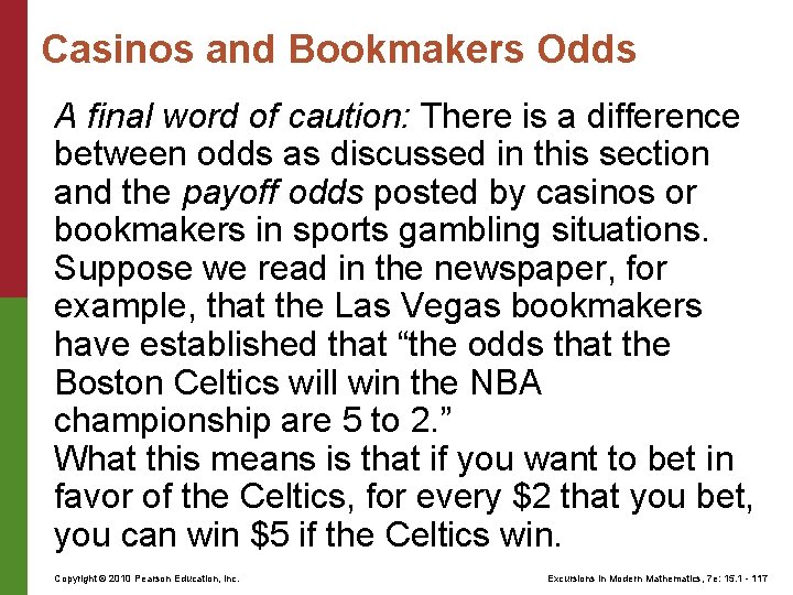
Casinos and Bookmakers Odds A final word of caution: There is a difference between odds as discussed in this section and the payoff odds posted by casinos or bookmakers in sports gambling situations. Suppose we read in the newspaper, for example, that the Las Vegas bookmakers have established that “the odds that the Boston Celtics will win the NBA championship are 5 to 2. ” What this means is that if you want to bet in favor of the Celtics, for every $2 that you bet, you can win $5 if the Celtics win. Copyright © 2010 Pearson Education, Inc. Excursions in Modern Mathematics, 7 e: 15. 1 - 117

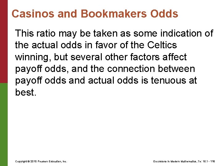
Casinos and Bookmakers Odds This ratio may be taken as some indication of the actual odds in favor of the Celtics winning, but several other factors affect payoff odds, and the connection between payoff odds and actual odds is tenuous at best. Copyright © 2010 Pearson Education, Inc. Excursions in Modern Mathematics, 7 e: 15. 1 - 118

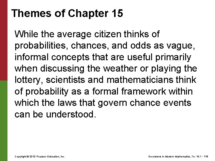
Themes of Chapter 15 While the average citizen thinks of probabilities, chances, and odds as vague, informal concepts that are useful primarily when discussing the weather or playing the lottery, scientists and mathematicians think of probability as a formal framework within which the laws that govern chance events can be understood. Copyright © 2010 Pearson Education, Inc. Excursions in Modern Mathematics, 7 e: 15. 1 - 119

Themes of Chapter 15 The basic elements of this framework are a sample space (which represents a precise mathematical description of all the possible outcomes of a random experiment), events (collections of these outcomes), and a probability assignment (which associates a numerical value to each of these events). Copyright © 2010 Pearson Education, Inc. Excursions in Modern Mathematics, 7 e: 15. 1 - 120

Themes of Chapter 15 Of the many ways in which probabilities can be assigned, a particularly important case is the one in which all individual outcomes have the same probability (equiprobable spaces). When this happens, the critical steps in calculating probabilities revolve around two basic (but not necessarily easy) questions: (1) What is the size of the sample space, and (2) what is the size of the event in question? To answer these kinds of questions, knowing the basic principles of “counting” is critical. Copyright © 2010 Pearson Education, Inc. Excursions in Modern Mathematics, 7 e: 15. 1 - 121

Themes of Chapter 15 When we stop to think how much of our lives is ruled by fate and chance, the importance of probability theory in almost every walk of life is hardly surprising. Understanding the basic mathematical principles behind this theory can help us better judge when taking a chance is a smart move and when it is not. In the long run, this will make us not just better card players, but also better and more successful citizens. Copyright © 2010 Pearson Education, Inc. Excursions in Modern Mathematics, 7 e: 15. 1 - 122