Transforming and Combining Random Variables LEARNING TARGETS By

Transforming and Combining Random Variables LEARNING TARGETS By the end of this section, you should be able to: üDESCRIBE the effect of adding or subtracting a constant or multiplying or dividing by a constant on the probability distribution of a random variable. üCALCULATE the mean and standard deviation of the sum or difference of random variables. üFIND probabilities involving the sum or difference of independent Normal random variables. Starnes/Tabor, The Practice of Statistics

Transforming a Random Variable In Chapter 2, we studied the effects of linear transformations on the shape, center, and variability of a distribution of data. Recall: 1. Adding (or subtracting) a constant a to each observation: • Adds (subtracts) a to measures of center and location. • Does not change the measures of variability. • Does not change the shape or measures of variability. 2. Multiplying (or dividing) each observation by a positive constant b: • Multiplies (divides) measures of center and location by b. • Multiplies (divides) measures of spread by b. • Does not change the shape of the distribution. Starnes/Tabor, The Practice of Statistics

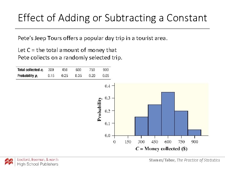
Effect of Adding or Subtracting a Constant Pete’s Jeep Tours offers a popular day trip in a tourist area. Let C = the total amount of money that Pete collects on a randomly selected trip. Starnes/Tabor, The Practice of Statistics

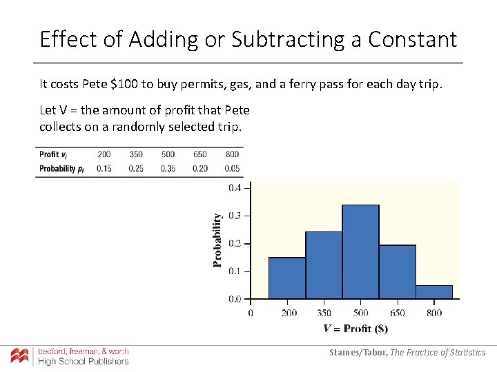
Effect of Adding or Subtracting a Constant It costs Pete $100 to buy permits, gas, and a ferry pass for each day trip. Let V = the amount of profit that Pete collects on a randomly selected trip. Starnes/Tabor, The Practice of Statistics

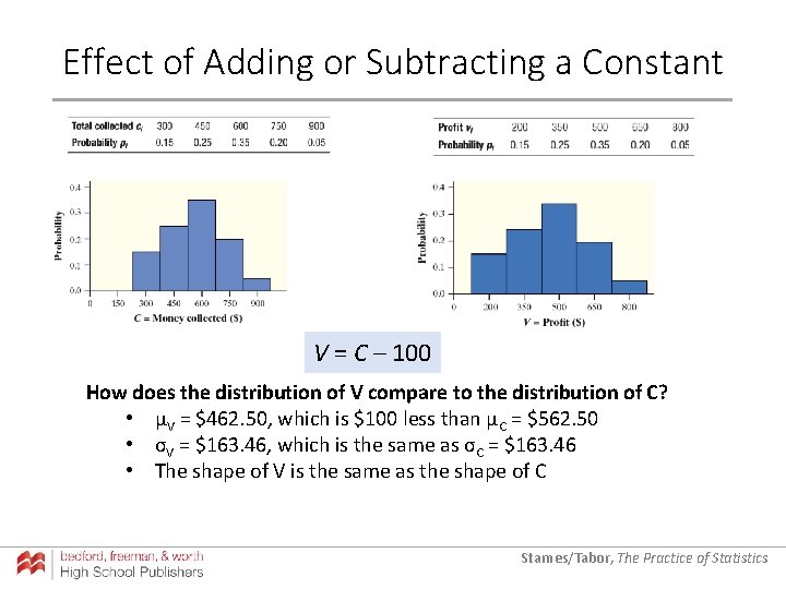
Effect of Adding or Subtracting a Constant V = C – 100 How does the distribution of V compare to the distribution of C? • µV = $462. 50, which is $100 less than µC = $562. 50 • σV = $163. 46, which is the same as σC = $163. 46 • The shape of V is the same as the shape of C Starnes/Tabor, The Practice of Statistics

Effect of Adding or Subtracting a Constant The Effect of Adding or Subtracting a Constant on a Probability Distribution Adding the same positive number a to (subtracting a from) each value of a random variable: • Adds a to (subtracts a from) measures of center and location (mean, median, quartiles, percentiles). • Does not change measures of variability (range, IQR, standard deviation). • Does not change the shape of the probability distribution. Note that adding or subtracting a constant affects the distribution of a quantitative variable and the probability distribution of a random variable in exactly the same way. Starnes/Tabor, The Practice of Statistics

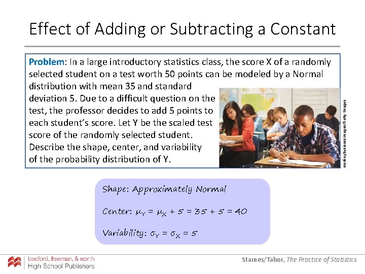
Problem: In a large introductory statistics class, the score X of a randomly selected student on a test worth 50 points can be modeled by a Normal distribution with mean 35 and standard deviation 5. Due to a difficult question on the test, the professor decides to add 5 points to each student’s score. Let Y be the scaled test score of the randomly selected student. Describe the shape, center, and variability of the probability distribution of Y. monkeybusinessimages/Getty Images Effect of Adding or Subtracting a Constant Shape: Approximately Normal Center: µY = µX + 5 = 35 + 5 = 40 Variability: σY = σX = 5 Starnes/Tabor, The Practice of Statistics

Effect of Multiplying or Dividing by a Constant The Effect of Multiplying or Dividing by a Constant on a Probability Distribution Multiplying (or dividing) each value of a random variable by the same positive number b: • Multiplies (divides) measures of center and location (mean, median, quartiles, percentiles) by b. • Multiplies (divides) measures of variability (range, IQR, standard deviation) by b. • Does not change the shape of the distribution. Multiplying or dividing by a constant has the same effect on the probability distribution of a random variable as it does on a distribution of quantitative data. Starnes/Tabor, The Practice of Statistics

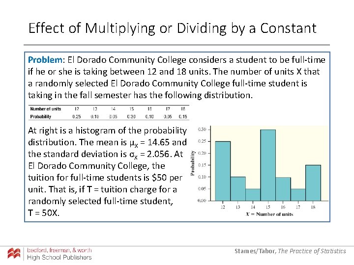
Effect of Multiplying or Dividing by a Constant Problem: El Dorado Community College considers a student to be full-time if he or she is taking between 12 and 18 units. The number of units X that a randomly selected El Dorado Community College full-time student is taking in the fall semester has the following distribution. At right is a histogram of the probability distribution. The mean is µX = 14. 65 and the standard deviation is σX = 2. 056. At El Dorado Community College, the tuition for full-time students is $50 per unit. That is, if T = tuition charge for a randomly selected full-time student, T = 50 X. Starnes/Tabor, The Practice of Statistics

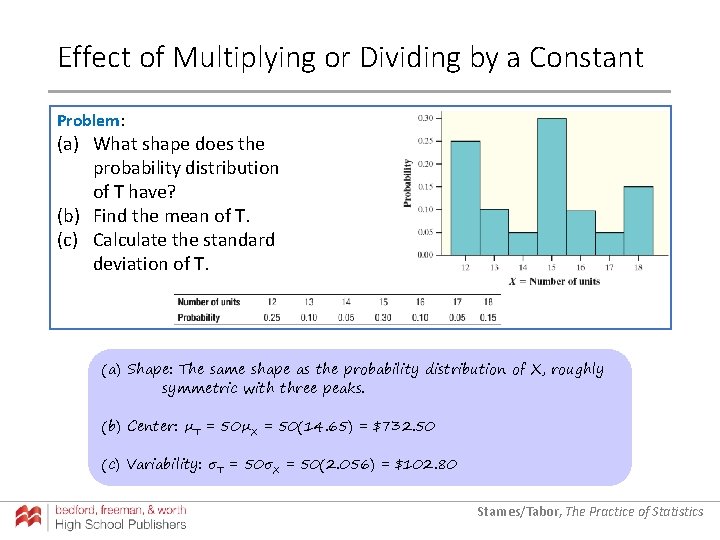
Effect of Multiplying or Dividing by a Constant Problem: (a) What shape does the probability distribution of T have? (b) Find the mean of T. (c) Calculate the standard deviation of T. (a) Shape: The same shape as the probability distribution of X, roughly symmetric with three peaks. (b) Center: µT = 50µX = 50(14. 65) = $732. 50 (c) Variability: σT = 50σX = 50(2. 056) = $102. 80 Starnes/Tabor, The Practice of Statistics

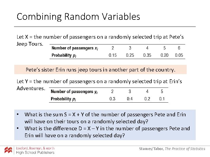
Combining Random Variables Let X = the number of passengers on a randomly selected trip at Pete’s Jeep Tours. Pete’s sister Erin runs jeep tours in another part of the country. Let Y = the number of passengers on a randomly selected trip at Erin’s Adventures. • What is the sum S = X + Y of the number of passengers Pete and Erin will have on their tours on a randomly selected day? • What is the difference D = X – Y in the number of passengers Pete and Erin will have on a randomly selected day? Starnes/Tabor, The Practice of Statistics

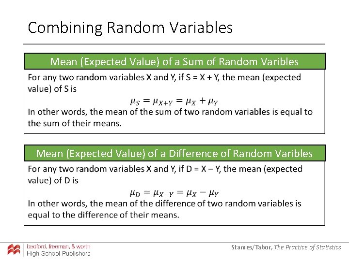
Combining Random Variables Mean (Expected Value) of a Sum of Random Varibles Mean (Expected Value) of a Difference of Random Varibles Starnes/Tabor, The Practice of Statistics

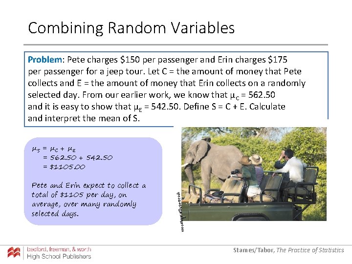
Combining Random Variables Problem: Pete charges $150 per passenger and Erin charges $175 per passenger for a jeep tour. Let C = the amount of money that Pete collects and E = the amount of money that Erin collects on a randomly selected day. From our earlier work, we know that µC = 562. 50 and it is easy to show that µE = 542. 50. Define S = C + E. Calculate and interpret the mean of S. /Superstoc moodboard Pete and Erin expect to collect a total of $1105 per day, on average, over many randomly selected days. k µS = µ C + µ E = 562. 50 + 542. 50 = $1105. 00 Starnes/Tabor, The Practice of Statistics

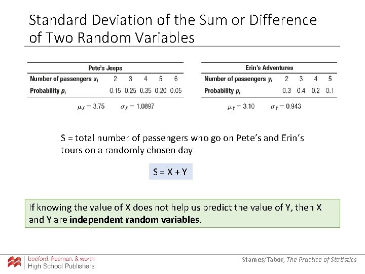
Standard Deviation of the Sum or Difference of Two Random Variables S = total number of passengers who go on Pete’s and Erin’s tours on a randomly chosen day S = X + Y If knowing the value of X does not help us predict the value of Y, then X and Y are independent random variables. Starnes/Tabor, The Practice of Statistics

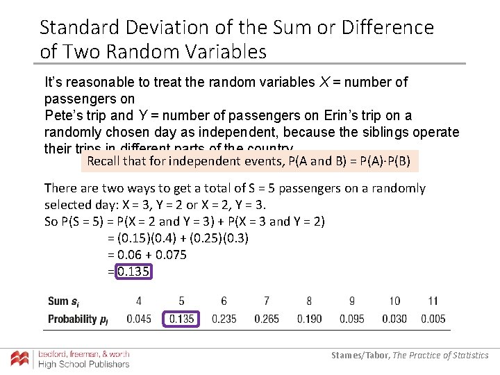
Standard Deviation of the Sum or Difference of Two Random Variables It’s reasonable to treat the random variables X = number of passengers on Pete’s trip and Y = number of passengers on Erin’s trip on a randomly chosen day as independent, because the siblings operate their trips in different parts of the country. Recall that for independent events, P(A and B) = P(A)·P(B) There are two ways to get a total of S = 5 passengers on a randomly selected day: X = 3, Y = 2 or X = 2, Y = 3. So P(S = 5) = P(X = 2 and Y = 3) + P(X = 3 and Y = 2) = (0. 15)(0. 4) + (0. 25)(0. 3) = 0. 06 + 0. 075 = 0. 135 Starnes/Tabor, The Practice of Statistics

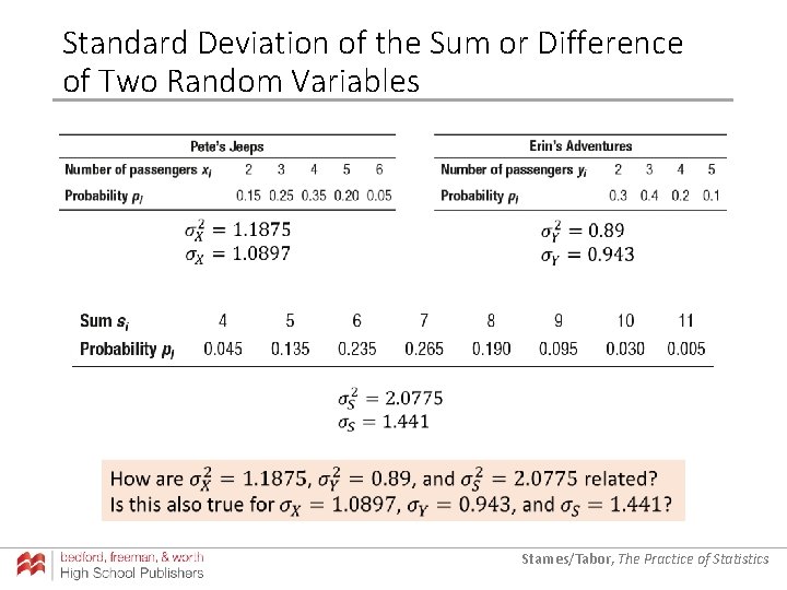
Standard Deviation of the Sum or Difference of Two Random Variables Starnes/Tabor, The Practice of Statistics

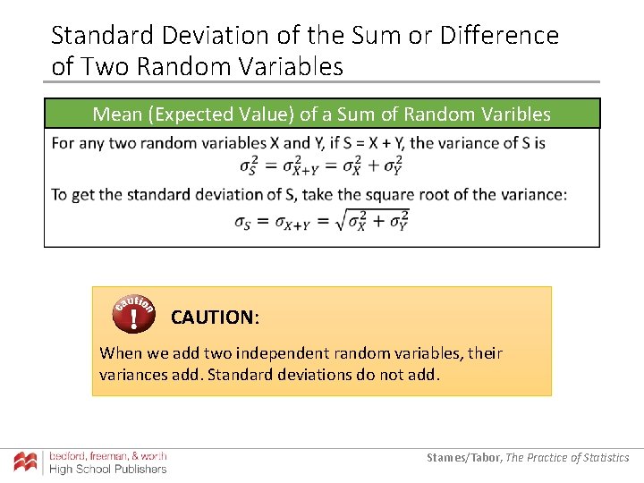
Standard Deviation of the Sum or Difference of Two Random Variables Mean (Expected Value) of a Sum of Random Varibles CAUTION: When we add two independent random variables, their variances add. Standard deviations do not add. Starnes/Tabor, The Practice of Statistics

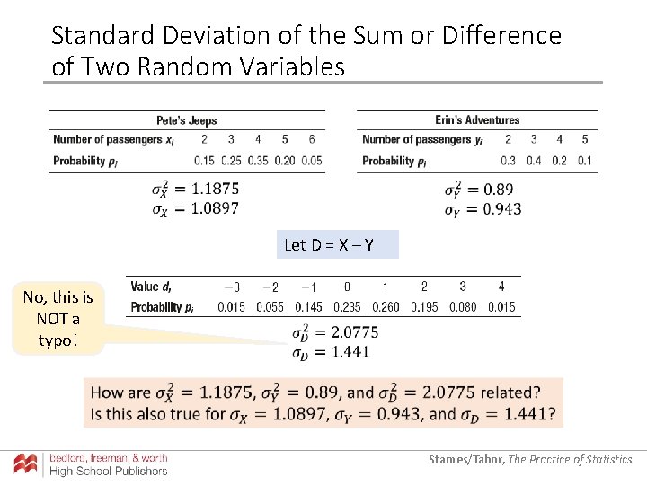
Standard Deviation of the Sum or Difference of Two Random Variables Let D = X – Y No, this is NOT a typo! Starnes/Tabor, The Practice of Statistics

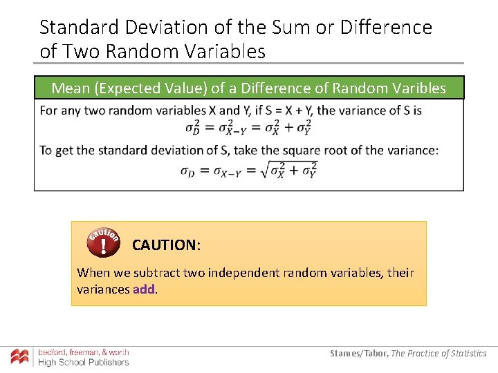
Standard Deviation of the Sum or Difference of Two Random Variables Mean (Expected Value) of a Difference of Random Varibles CAUTION: When we subtract two independent random variables, their variances add. Starnes/Tabor, The Practice of Statistics

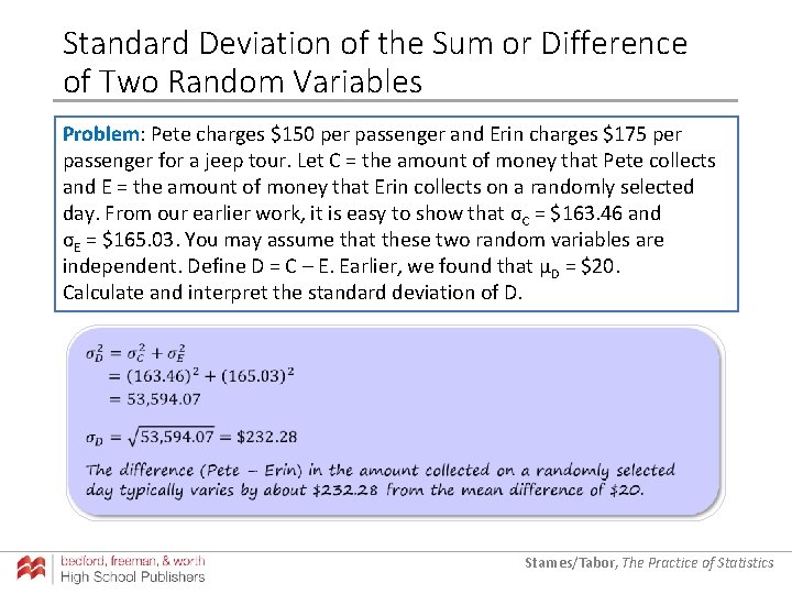
Standard Deviation of the Sum or Difference of Two Random Variables Problem: Pete charges $150 per passenger and Erin charges $175 per passenger for a jeep tour. Let C = the amount of money that Pete collects and E = the amount of money that Erin collects on a randomly selected day. From our earlier work, it is easy to show that σC = $163. 46 and σE = $165. 03. You may assume that these two random variables are independent. Define D = C – E. Earlier, we found that µD = $20. Calculate and interpret the standard deviation of D. Starnes/Tabor, The Practice of Statistics

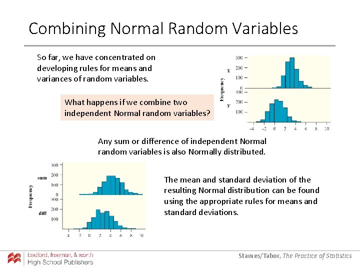
Combining Normal Random Variables So far, we have concentrated on developing rules for means and variances of random variables. What happens if we combine two independent Normal random variables? Any sum or difference of independent Normal random variables is also Normally distributed. The mean and standard deviation of the resulting Normal distribution can be found using the appropriate rules for means and standard deviations. Starnes/Tabor, The Practice of Statistics

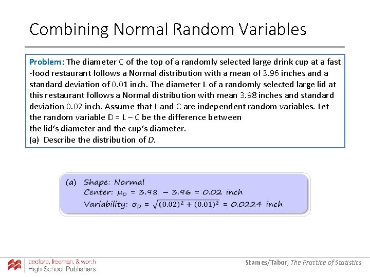
Combining Normal Random Variables Problem: The diameter C of the top of a randomly selected large drink cup at a fast -food restaurant follows a Normal distribution with a mean of 3. 96 inches and a standard deviation of 0. 01 inch. The diameter L of a randomly selected large lid at this restaurant follows a Normal distribution with mean 3. 98 inches and standard deviation 0. 02 inch. Assume that L and C are independent random variables. Let the random variable D = L – C be the difference between the lid’s diameter and the cup’s diameter. (a) Describe the distribution of D. Starnes/Tabor, The Practice of Statistics

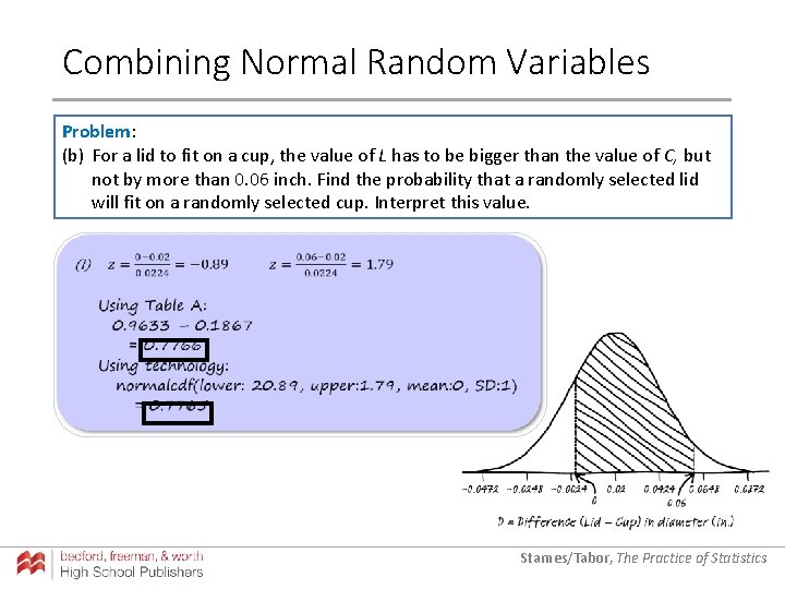
Combining Normal Random Variables Problem: (b) For a lid to fit on a cup, the value of L has to be bigger than the value of C, but not by more than 0. 06 inch. Find the probability that a randomly selected lid will fit on a randomly selected cup. Interpret this value. Starnes/Tabor, The Practice of Statistics

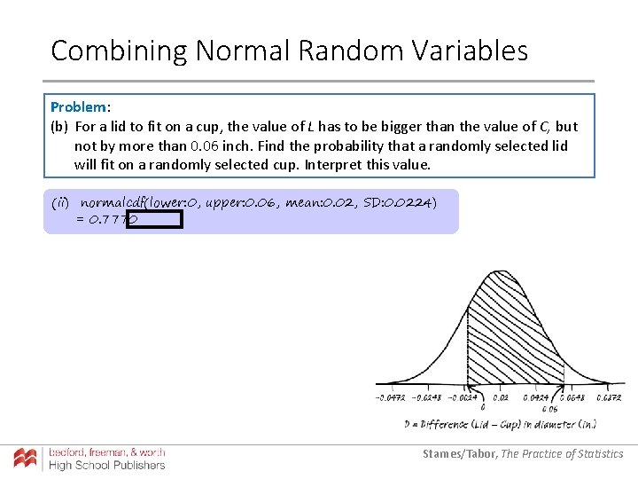
Combining Normal Random Variables Problem: (b) For a lid to fit on a cup, the value of L has to be bigger than the value of C, but not by more than 0. 06 inch. Find the probability that a randomly selected lid will fit on a randomly selected cup. Interpret this value. (ii) normalcdf(lower: 0, upper: 0. 06, mean: 0. 02, SD: 0. 0224) = 0. 7770 Starnes/Tabor, The Practice of Statistics

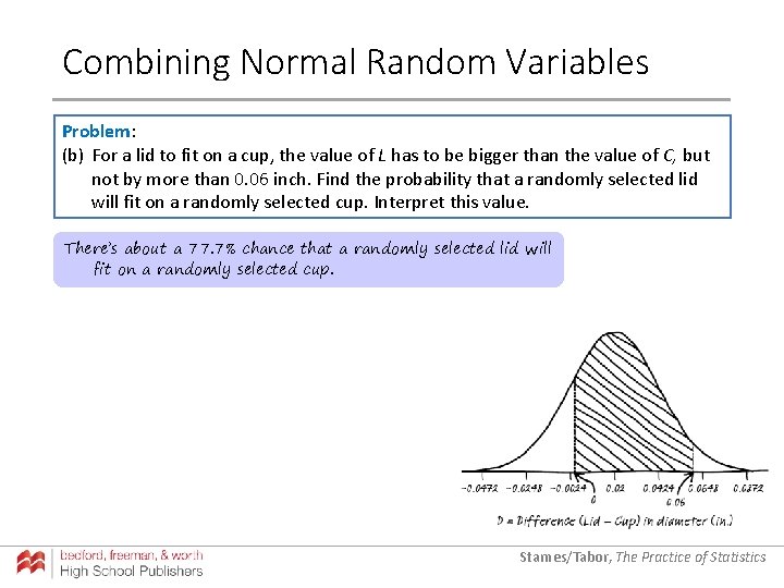
Combining Normal Random Variables Problem: (b) For a lid to fit on a cup, the value of L has to be bigger than the value of C, but not by more than 0. 06 inch. Find the probability that a randomly selected lid will fit on a randomly selected cup. Interpret this value. There’s about a 77. 7% chance that a randomly selected lid will fit on a randomly selected cup. Starnes/Tabor, The Practice of Statistics