Random Walk Models for Stock Prices Statistics and

Random Walk Models for Stock Prices Statistics and Data Analysis Professor William Greene Stern School of Business Department of IOMS Department of Economics

Random Walk Models for Stock Prices Statistics and Data Analysis Random Walk Models for Stock Prices

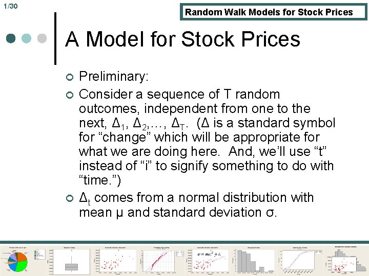
1/30 Random Walk Models for Stock Prices A Model for Stock Prices ¢ ¢ ¢ Preliminary: Consider a sequence of T random outcomes, independent from one to the next, Δ 1, Δ 2, …, ΔT. (Δ is a standard symbol for “change” which will be appropriate for what we are doing here. And, we’ll use “t” instead of “i” to signify something to do with “time. ”) Δt comes from a normal distribution with mean μ and standard deviation σ.

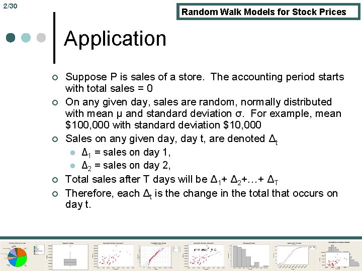
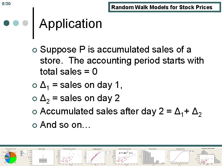
2/30 Random Walk Models for Stock Prices Application ¢ ¢ ¢ Suppose P is sales of a store. The accounting period starts with total sales = 0 On any given day, sales are random, normally distributed with mean μ and standard deviation σ. For example, mean $100, 000 with standard deviation $10, 000 Sales on any given day, day t, are denoted Δt l Δ 1 = sales on day 1, l Δ 2 = sales on day 2, Total sales after T days will be Δ 1+ Δ 2+…+ ΔT Therefore, each Δt is the change in the total that occurs on day t.

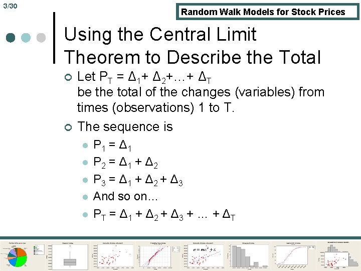
3/30 Random Walk Models for Stock Prices Using the Central Limit Theorem to Describe the Total ¢ ¢ Let PT = Δ 1+ Δ 2+…+ ΔT be the total of the changes (variables) from times (observations) 1 to T. The sequence is l l l P 1 = Δ 1 P 2 = Δ 1 + Δ 2 P 3 = Δ 1 + Δ 2 + Δ 3 And so on… PT = Δ 1 + Δ 2 + Δ 3 + … + ΔT

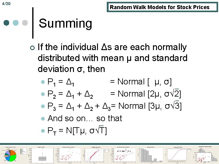
4/30 Random Walk Models for Stock Prices Summing ¢ If the individual Δs are each normally distributed with mean μ and standard deviation σ, then P 1 = Δ 1 = Normal [ μ, σ] l P 2 = Δ 1 + Δ 2 = Normal [2μ, σ√ 2] l P 3 = Δ 1 + Δ 2 + Δ 3= Normal [3μ, σ√ 3] l And so on… so that l PT = N[Tμ, σ√T] l

5/30 Random Walk Models for Stock Prices Application Suppose P is accumulated sales of a store. The accounting period starts with total sales = 0 ¢ Δ 1 = sales on day 1, ¢ Δ 2 = sales on day 2 ¢ Accumulated sales after day 2 = Δ 1+ Δ 2 ¢ And so on… ¢

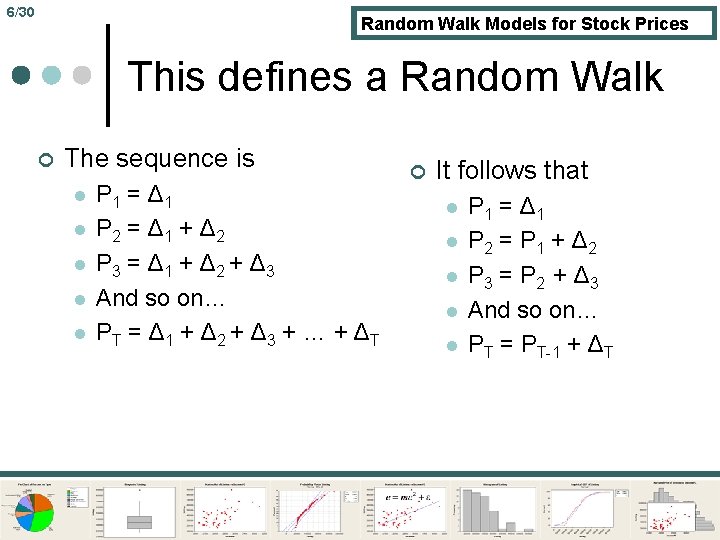
6/30 Random Walk Models for Stock Prices This defines a Random Walk ¢ The sequence is l l l P 1 = Δ 1 P 2 = Δ 1 + Δ 2 P 3 = Δ 1 + Δ 2 + Δ 3 And so on… PT = Δ 1 + Δ 2 + Δ 3 + … + ΔT ¢ It follows that l l l P 1 = Δ 1 P 2 = P 1 + Δ 2 P 3 = P 2 + Δ 3 And so on… PT = PT-1 + ΔT

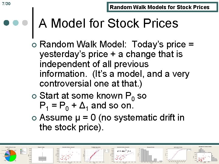
7/30 Random Walk Models for Stock Prices A Model for Stock Prices Random Walk Model: Today’s price = yesterday’s price + a change that is independent of all previous information. (It’s a model, and a very controversial one at that. ) ¢ Start at some known P 0 so P 1 = P 0 + Δ 1 and so on. ¢ Assume μ = 0 (no systematic drift in the stock price). ¢

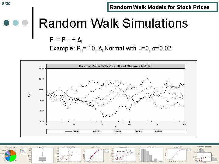
8/30 Random Walk Models for Stock Prices Random Walk Simulations Pt = Pt-1 + Δt Example: P 0= 10, Δt Normal with μ=0, σ=0. 02

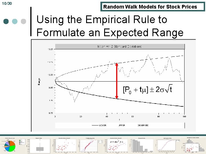
9/30 Random Walk Models for Stock Prices Uncertainty Expected Price = E[Pt] = P 0+Tμ We have used μ = 0 (no systematic upward or downward drift). ¢ Standard deviation = σ√T reflects uncertainty. ¢ Looking forward from “now” = time t=0, the uncertainty increases the farther out we look to the future. ¢

10/30 Random Walk Models for Stock Prices Using the Empirical Rule to Formulate an Expected Range

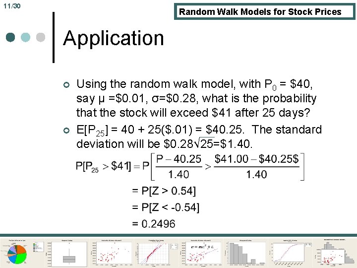
11/30 Random Walk Models for Stock Prices Application ¢ ¢ Using the random walk model, with P 0 = $40, say μ =$0. 01, σ=$0. 28, what is the probability that the stock will exceed $41 after 25 days? E[P 25] = 40 + 25($. 01) = $40. 25. The standard deviation will be $0. 28√ 25=$1. 40.

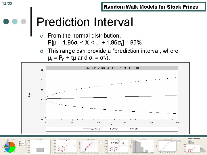
12/30 Random Walk Models for Stock Prices Prediction Interval ¢ ¢ From the normal distribution, P[μt - 1. 96σt < X < μt + 1. 96σt] = 95% This range can provide a “prediction interval, where μt = P 0 + tμ and σt = σ√t.

13/30 Random Walk Models for Stock Prices Random Walk Model ¢ ¢ ¢ Controversial – many assumptions l Normality is inessential – we are summing, so after 25 periods or so, we can invoke the CLT. l The assumption of period to period independence is at least debatable. l The assumption of unchanging mean and variance is certainly debatable. The additive model allows negative prices. (Ouch!) The model when applied is usually based on logs and the lognormal model. To be continued …

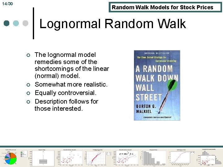
14/30 Random Walk Models for Stock Prices Lognormal Random Walk ¢ ¢ The lognormal model remedies some of the shortcomings of the linear (normal) model. Somewhat more realistic. Equally controversial. Description follows for those interested.

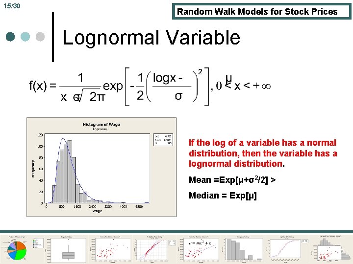
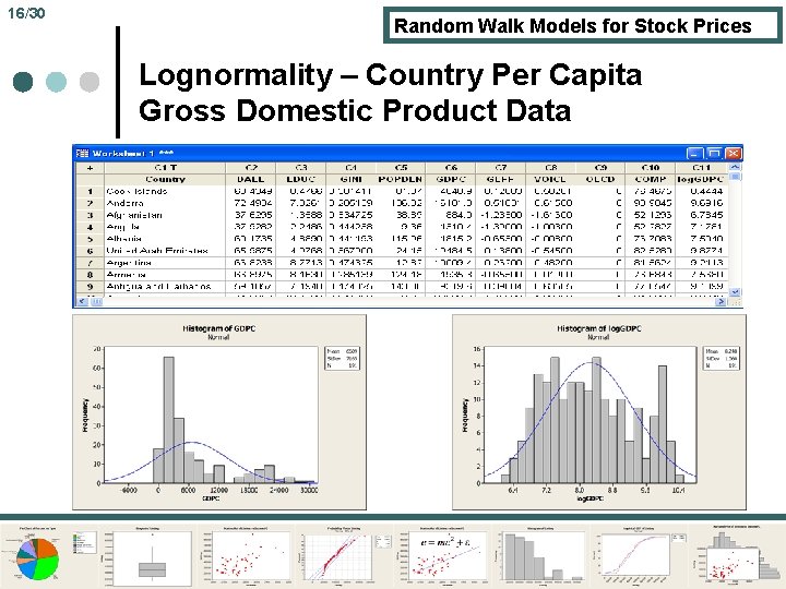
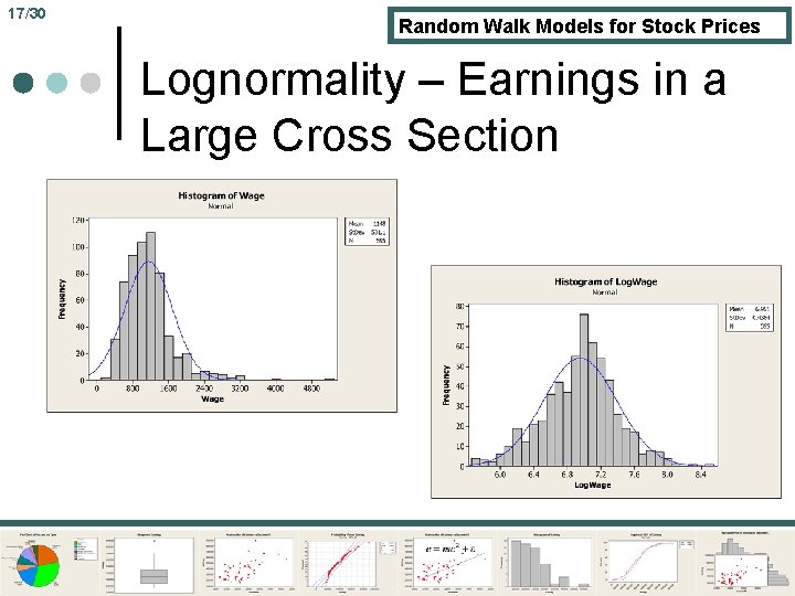
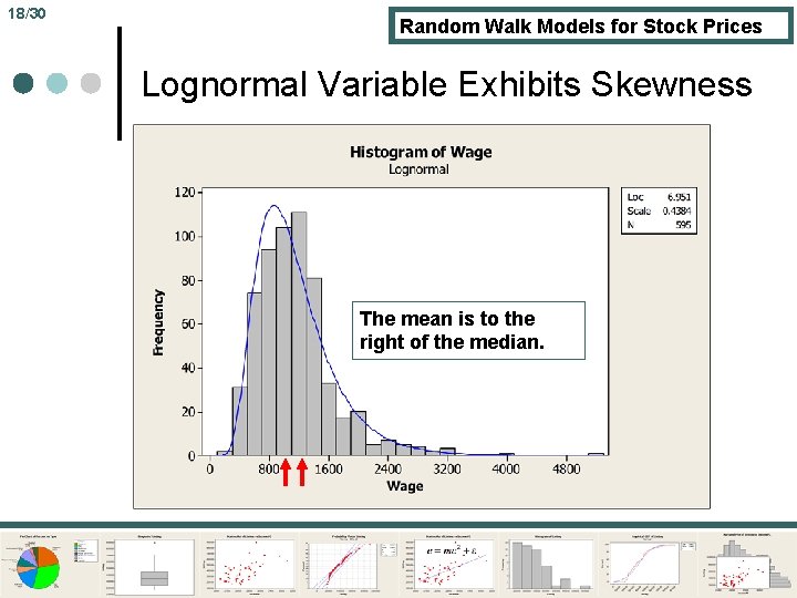
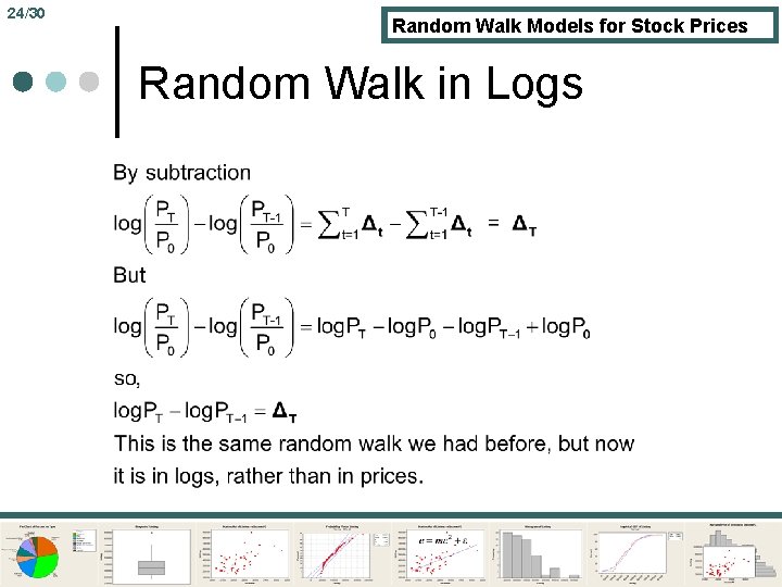
15/30 Random Walk Models for Stock Prices Lognormal Variable If the log of a variable has a normal distribution, then the variable has a lognormal distribution. Mean =Exp[μ+σ2/2] > Median = Exp[μ]

16/30 Random Walk Models for Stock Prices Lognormality – Country Per Capita Gross Domestic Product Data

17/30 Random Walk Models for Stock Prices Lognormality – Earnings in a Large Cross Section

18/30 Random Walk Models for Stock Prices Lognormal Variable Exhibits Skewness The mean is to the right of the median.

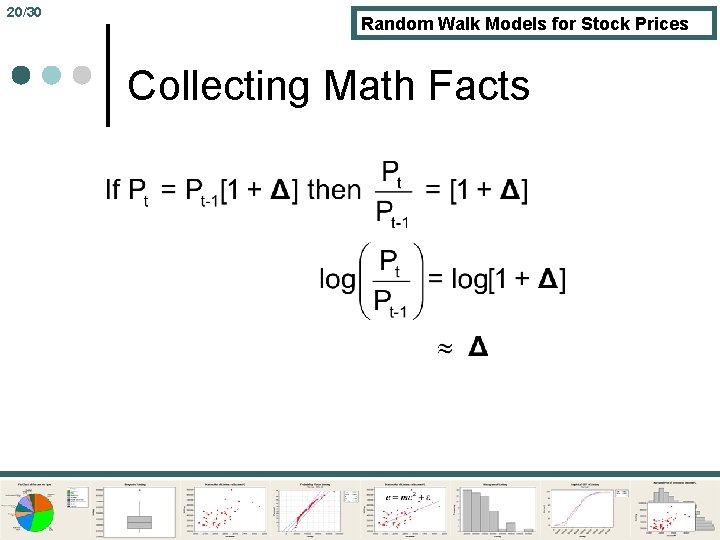
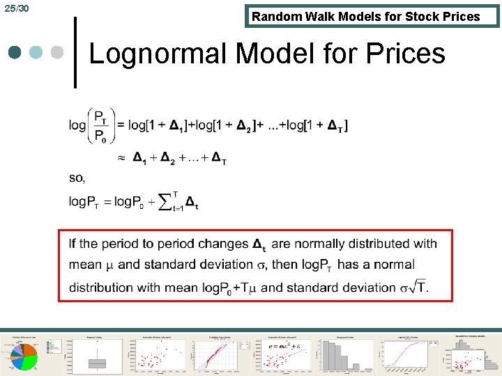
19/30 Random Walk Models for Stock Prices Lognormal Distribution for Price Changes ¢ ¢ Math preliminaries: (Growth) If price is P 0 at time 0 and the price grows by 100Δ% from period 0 to period 1, then the price at period 1 is P 0(1 + Δ). For example, P 0=40; Δ = 0. 04 (4% period); P 1 = P 0(1 + 0. 04). ¢ (Price ratio) If P 1 = P 0(1 + 0. 04) then P 1/P 0 = (1 + 0. 04). ¢ (Math fact) For smallish Δ, log(1 + Δ) ≈ Δ Example, if Δ = 0. 04, log(1 + 0. 04) = 0. 39221.

20/30 Random Walk Models for Stock Prices Collecting Math Facts

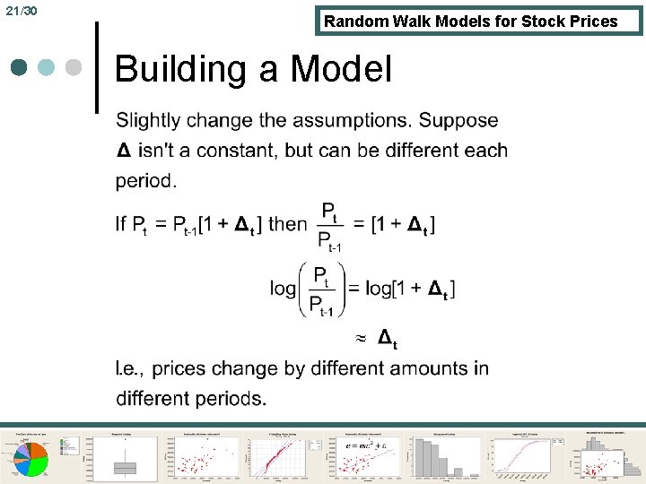
21/30 Random Walk Models for Stock Prices Building a Model

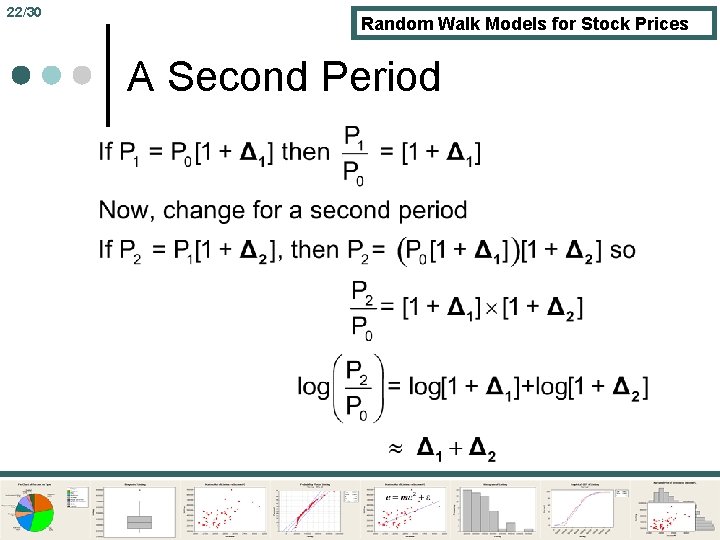
22/30 Random Walk Models for Stock Prices A Second Period

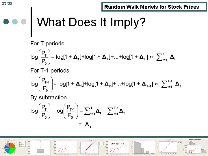
23/30 Random Walk Models for Stock Prices What Does It Imply?

24/30 Random Walk Models for Stock Prices Random Walk in Logs

25/30 Random Walk Models for Stock Prices Lognormal Model for Prices

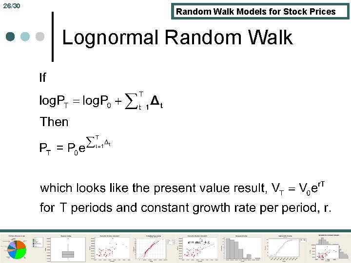
26/30 Random Walk Models for Stock Prices Lognormal Random Walk

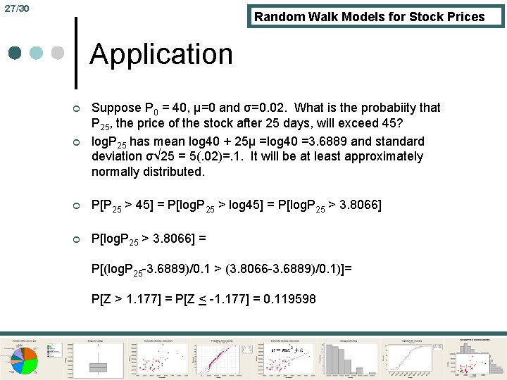
27/30 Random Walk Models for Stock Prices Application ¢ Suppose P 0 = 40, μ=0 and σ=0. 02. What is the probabiity that P 25, the price of the stock after 25 days, will exceed 45? log. P 25 has mean log 40 + 25μ =log 40 =3. 6889 and standard deviation σ√ 25 = 5(. 02)=. 1. It will be at least approximately normally distributed. ¢ P[P 25 > 45] = P[log. P 25 > log 45] = P[log. P 25 > 3. 8066] ¢ P[log. P 25 > 3. 8066] = ¢ P[(log. P 25 -3. 6889)/0. 1 > (3. 8066 -3. 6889)/0. 1)]= P[Z > 1. 177] = P[Z < -1. 177] = 0. 119598

28/30 Random Walk Models for Stock Prices Prediction Interval We are 95% certain that log. P 25 is in the interval log. P 0 + μ 25 - 1. 96σ25 to log. P 0 + μ 25 + 1. 96σ25. Continue to assume μ=0 so μ 25 = 25(0)=0 and σ=0. 02 so σ25 = 0. 02(√ 25)=0. 1 Then, the interval is 3. 6889 -1. 96(0. 1) to 3. 6889 + 1. 96(0. 1) or 3. 4929 to 3. 8849. This means that we are 95% confident that P 0 is in the range e 3. 4929 = 32. 88 and e 3. 8849 = 48. 66

29/30 Random Walk Models for Stock Prices Observations - 1 The lognormal model (lognormal random walk) predicts that the price will always take the form PT = P 0 eΣΔt ¢ This will always be positive, so this overcomes the problem of the first model we looked at. ¢

30/30 Random Walk Models for Stock Prices Observations - 2 ¢ ¢ The lognormal model has a quirk of its own. Note that when we formed the prediction interval for P 25 based on P 0 = 40, the interval is [32. 88, 48. 66] which has center at 40. 77 > 40, even though μ = 0. It looks like free money. Why does this happen? A feature of the lognormal model is that E[PT] = P 0 exp(μT + ½σT 2) which is greater than P 0 even if μ = 0. Philosophically, we can interpret this as the expected return to undertaking risk (compared to no risk – a risk “premium”). On the other hand, this is a model. It has virtues and flaws. This is one of the flaws.