Chapter 10 Curve Fitting and Regression Analysis Correlation

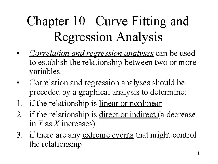
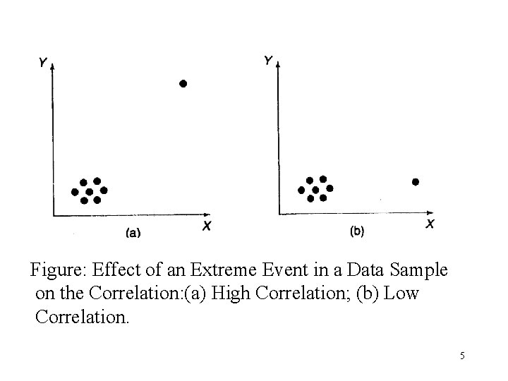
Chapter 10 Curve Fitting and Regression Analysis • Correlation and regression analyses can be used to establish the relationship between two or more variables. • Correlation and regression analyses should be preceded by a graphical analysis to determine: 1. if the relationship is linear or nonlinear 2. if the relationship is direct or indirect (a decrease in Y as X increases) 3. if there any extreme events that might control the relationship 1

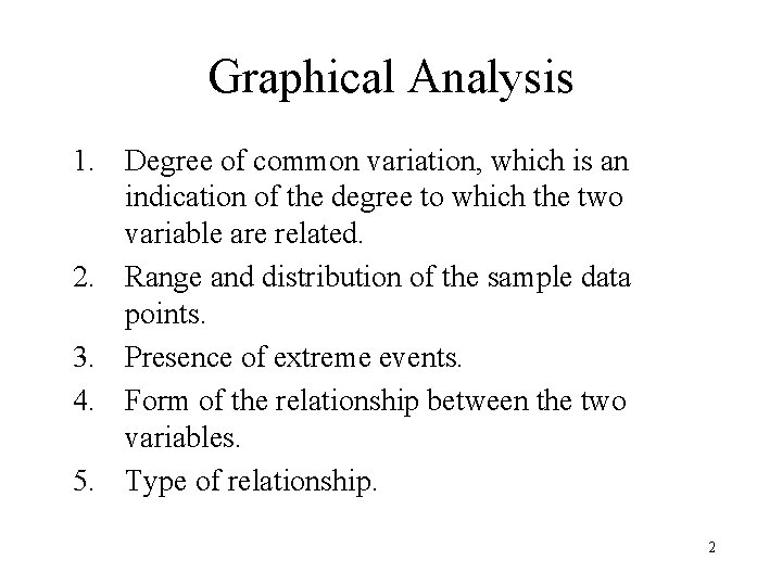
Graphical Analysis 1. Degree of common variation, which is an indication of the degree to which the two variable are related. 2. Range and distribution of the sample data points. 3. Presence of extreme events. 4. Form of the relationship between the two variables. 5. Type of relationship. 2

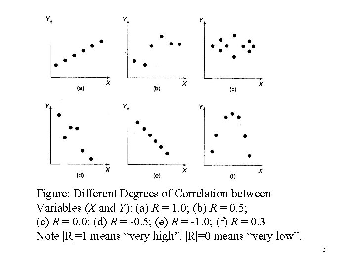
Figure: Different Degrees of Correlation between Variables (X and Y): (a) R = 1. 0; (b) R = 0. 5; (c) R = 0. 0; (d) R = -0. 5; (e) R = -1. 0; (f) R = 0. 3. Note |R|=1 means “very high”. |R|=0 means “very low”. 3

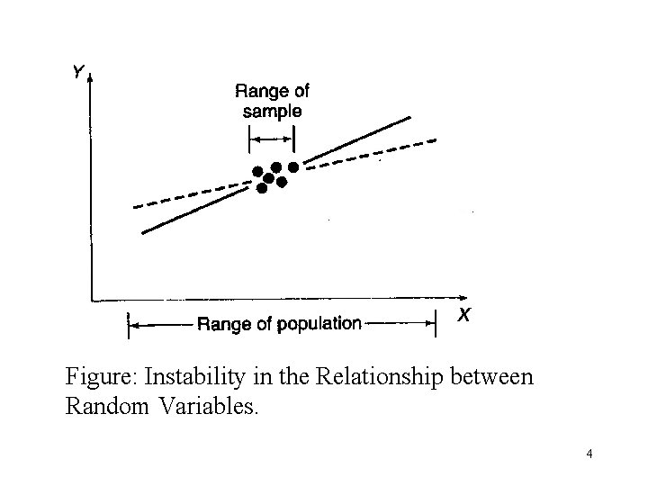
Figure: Instability in the Relationship between Random Variables. 4

Figure: Effect of an Extreme Event in a Data Sample on the Correlation: (a) High Correlation; (b) Low Correlation. 5

Correlation Analysis • Correlation is the degree of association between two variables. • Correlation analysis provides a quantitative index of the degree to which one or more variables can be used to predict the values of another variable. • Correlation analyses are most often performed after an equation relating one variable to another has been developed. 6

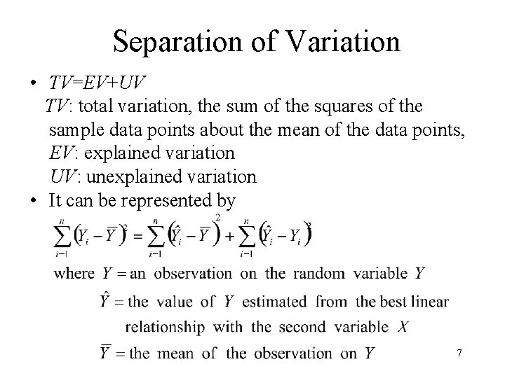
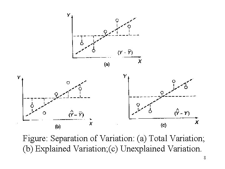
Separation of Variation • TV=EV+UV TV: total variation, the sum of the squares of the sample data points about the mean of the data points, EV: explained variation UV: unexplained variation • It can be represented by 7

Figure: Separation of Variation: (a) Total Variation; (b) Explained Variation; (c) Unexplained Variation. 8

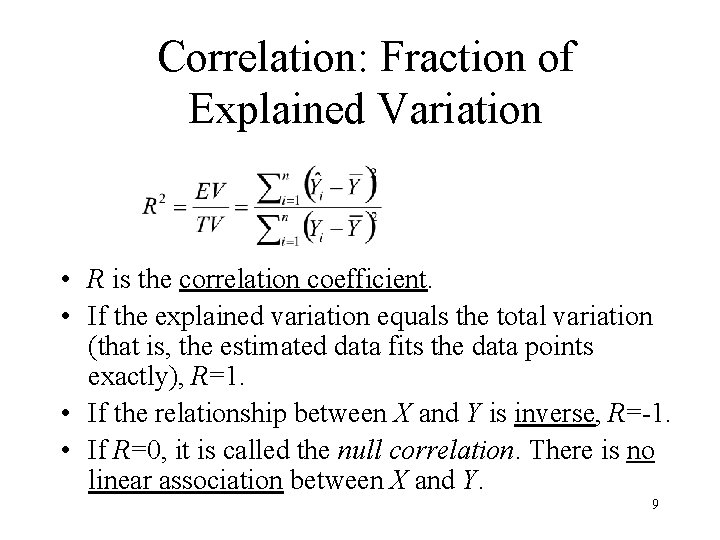
Correlation: Fraction of Explained Variation • R is the correlation coefficient. • If the explained variation equals the total variation (that is, the estimated data fits the data points exactly), R=1. • If the relationship between X and Y is inverse, R=-1. • If R=0, it is called the null correlation. There is no linear association between X and Y. 9

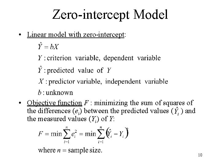
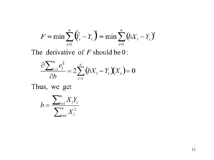
Zero-intercept Model • Linear model with zero-intercept: • Objective function F : minimizing the sum of squares of the differences (ei) between the predicted values ( ) and the measured values (Yi) of Y: 10

11

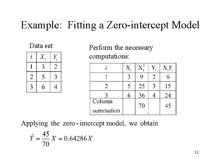
Example: Fitting a Zero-intercept Model Data set Perform the necessary computations: 12

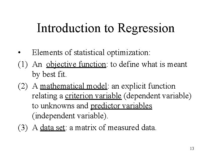
Introduction to Regression • Elements of statistical optimization: (1) An objective function: to define what is meant by best fit. (2) A mathematical model: an explicit function relating a criterion variable (dependent variable) to unknowns and predictor variables (independent variable). (3) A data set: a matrix of measured data. 13

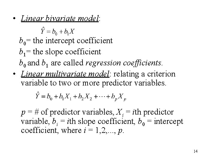
• Linear bivariate model: b 0= the intercept coefficient b 1= the slope coefficient b 0 and b 1 are called regression coefficients. • Linear multivariate model: relating a criterion variable to two or more predictor variables. p = # of predictor variables, Xi = ith predictor variable, bi = ith slope coefficient, b 0 = intercept coefficient, where i = 1, 2, . . . , p. 14

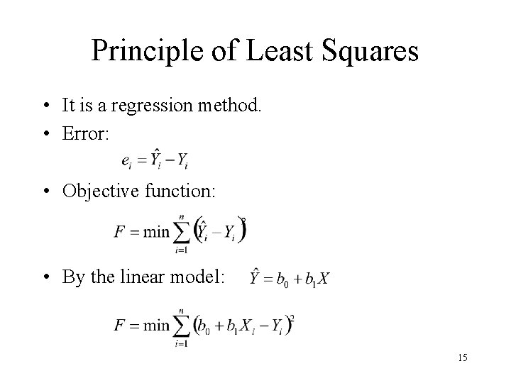
Principle of Least Squares • It is a regression method. • Error: • Objective function: • By the linear model: 15

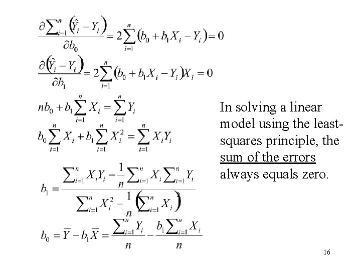
In solving a linear model using the leastsquares principle, the sum of the errors always equals zero. 16

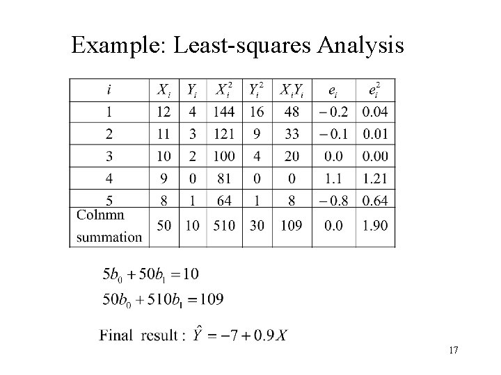
Example: Least-squares Analysis 17

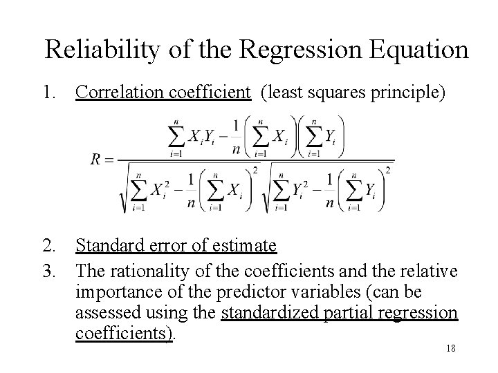
Reliability of the Regression Equation 1. Correlation coefficient (least squares principle) 2. Standard error of estimate 3. The rationality of the coefficients and the relative importance of the predictor variables (can be assessed using the standardized partial regression coefficients). 18

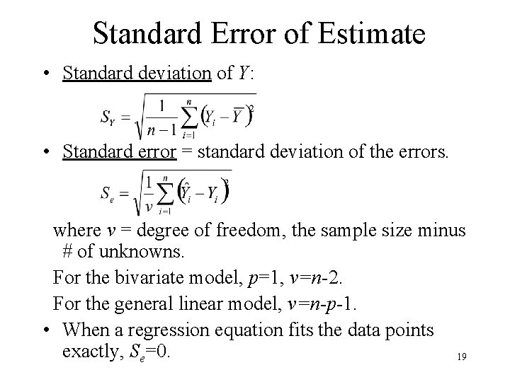
Standard Error of Estimate • Standard deviation of Y: • Standard error = standard deviation of the errors. where v = degree of freedom, the sample size minus # of unknowns. For the bivariate model, p=1, v=n-2. For the general linear model, v=n-p-1. • When a regression equation fits the data points exactly, Se=0. 19

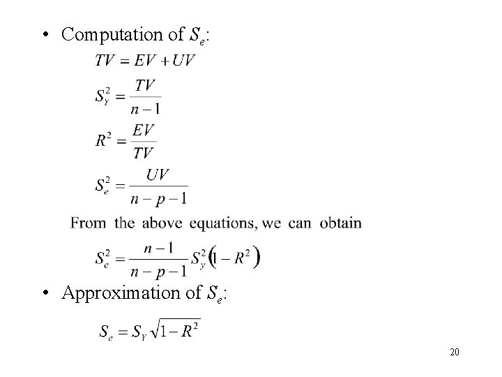
• Computation of Se: • Approximation of Se: 20

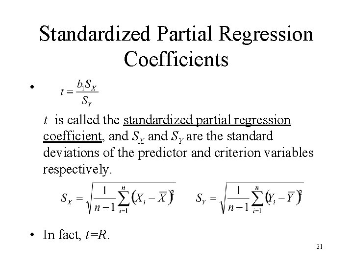
Standardized Partial Regression Coefficients • t is called the standardized partial regression coefficient, and SX and SY are the standard deviations of the predictor and criterion variables respectively. • In fact, t=R. 21

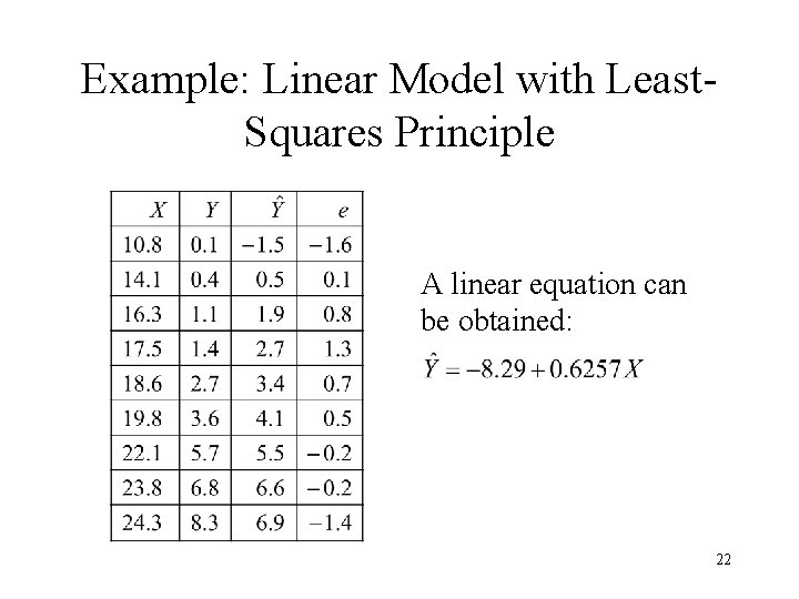
Example: Linear Model with Least. Squares Principle A linear equation can be obtained: 22

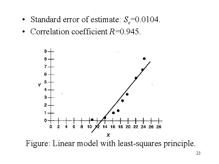
• Standard error of estimate: Se=0. 0104. • Correlation coefficient R=0. 945. Figure: Linear model with least-squares principle. 23

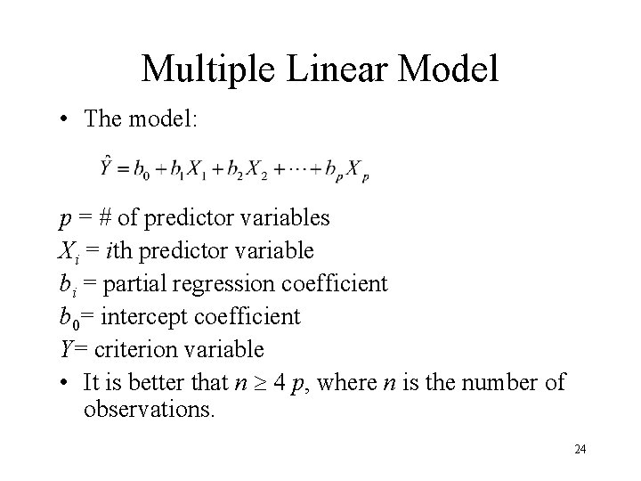
Multiple Linear Model • The model: p = # of predictor variables Xi = ith predictor variable bi = partial regression coefficient b 0= intercept coefficient Y= criterion variable • It is better that n 4 p, where n is the number of observations. 24

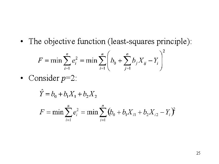
• The objective function (least-squares principle): • Consider p=2: 25

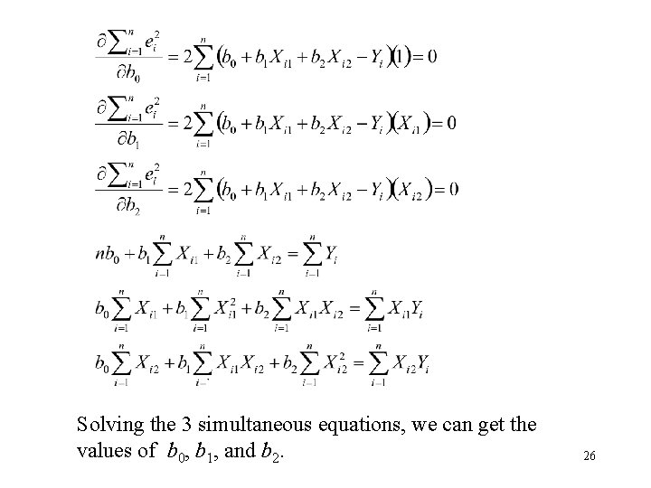
Solving the 3 simultaneous equations, we can get the values of b 0, b 1, and b 2. 26

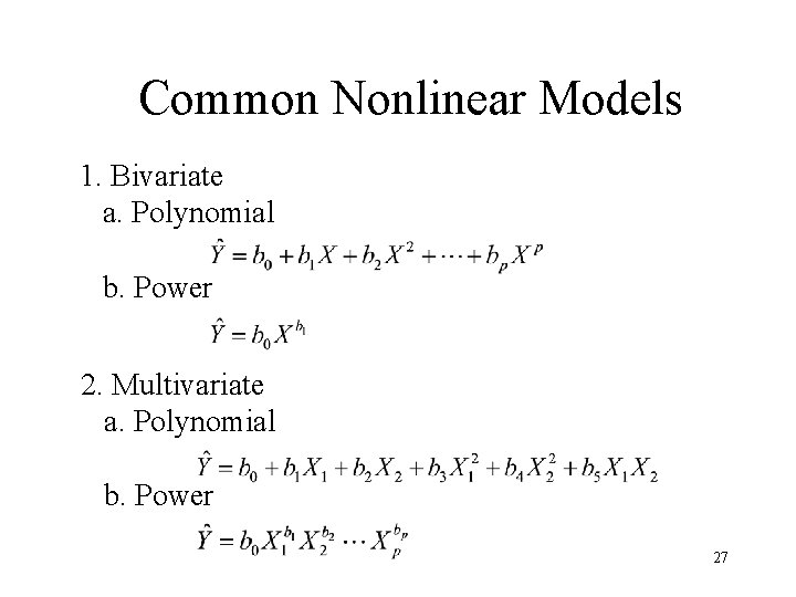
Common Nonlinear Models 1. Bivariate a. Polynomial b. Power 2. Multivariate a. Polynomial b. Power 27

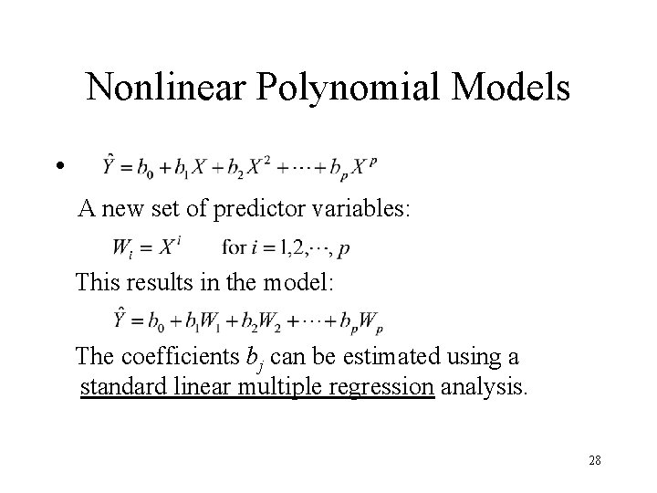
Nonlinear Polynomial Models • A new set of predictor variables: This results in the model: The coefficients bj can be estimated using a standard linear multiple regression analysis. 28

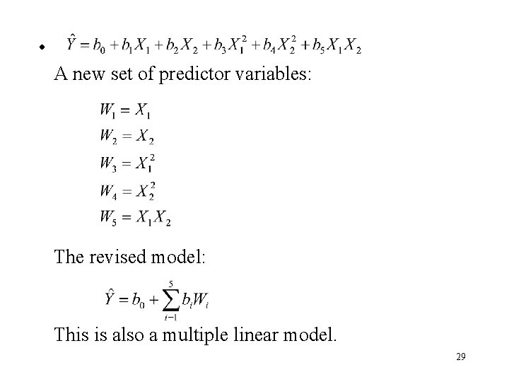
• A new set of predictor variables: The revised model: This is also a multiple linear model. 29

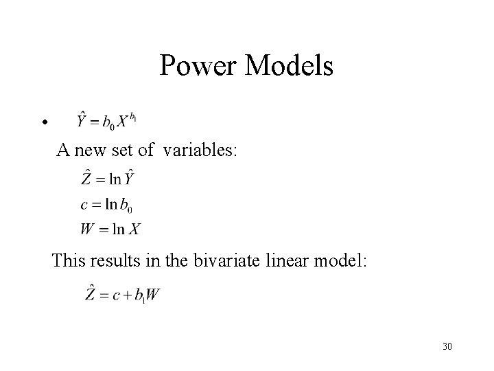
Power Models • A new set of variables: This results in the bivariate linear model: 30

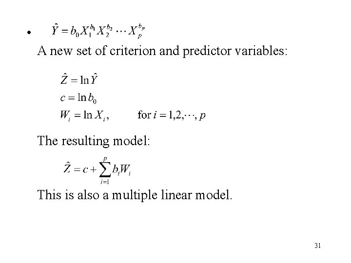
• A new set of criterion and predictor variables: The resulting model: This is also a multiple linear model. 31

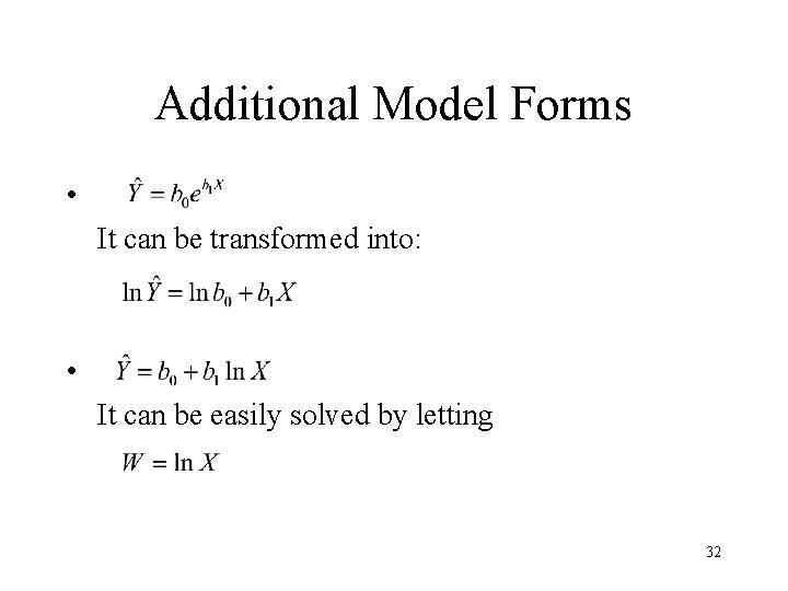
Additional Model Forms • It can be transformed into: • It can be easily solved by letting 32