Causal Inference and Graphical Models Peter Spirtes Carnegie

Causal Inference and Graphical Models Peter Spirtes Carnegie Mellon University

Overview Manipulations l Assuming no Hidden Common Causes l From DAGs to Effects of Manipulation n From Data to Sets of DAGs n From Sets of Dags to Effects of Manipulation n l May be Hidden Common Causes From Data to Sets of DAGs n From Sets of DAGs to Effects of Manipulations n

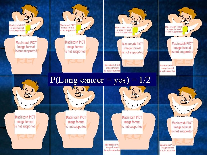
If I were to force a group of people to smoke one pack a day, what percentage would develop lung cancer? The Evidence

P(Lung cancer = yes) = 1/2

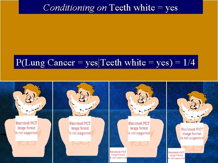
Conditioning on Teeth white = yes P(Lung Cancer = yes|Teeth white = yes) = 1/4

Manipulating Teeth white = yes

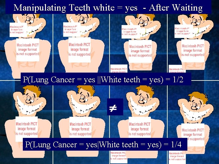
Manipulating Teeth white = yes - After Waiting P(Lung Cancer = yes ||White teeth = yes) = 1/2 P(Lung Cancer = yes|White teeth = yes) = 1/4

Smoking Decision Setting insurance rates for smokers - conditioning l Suppose the Surgeon General is considering banning smoking? l Will this decrease smoking? n Will decreasing smoking decrease cancer? n Will it have negative side-effects – e. g. more obesity? n How is greater life expectancy valued against decrease in pleasure from smoking? n

Manipulations and Distributions l Since Smoking determines Teeth white, P(T, L, R, W) = P(S, L, R, W) l But the manipulation of Teeth white leads to different results than the manipulation of Smoking l Hence the distribution does not always uniquely determine the results of a manipulation

Causation l We will infer average causal effects. n We will not consider quantities such as probability of necessity, probability of sufficiency, or the counterfactual probability that I would get a headache conditional on taking an aspirin, given that I did not take an aspirin The causal relations are between properties of a unit at a time, not between events. l Each unit is assumed to be causally isolated. l The causal relations may be genuinely indeterministic, or only apparently indeterministic. l

Causal DAGs l Probabilistic Interpretation of DAGs n. A DAG represents a distribution P when each variable is independent of its nondescendants conditional on its parents in the DAG l Causal n There Interpretation of DAGs is a directed edge from A to B (relative to V) when A is a direct cause of B. n An acyclic graph is not a representation of reversible or feedback processes

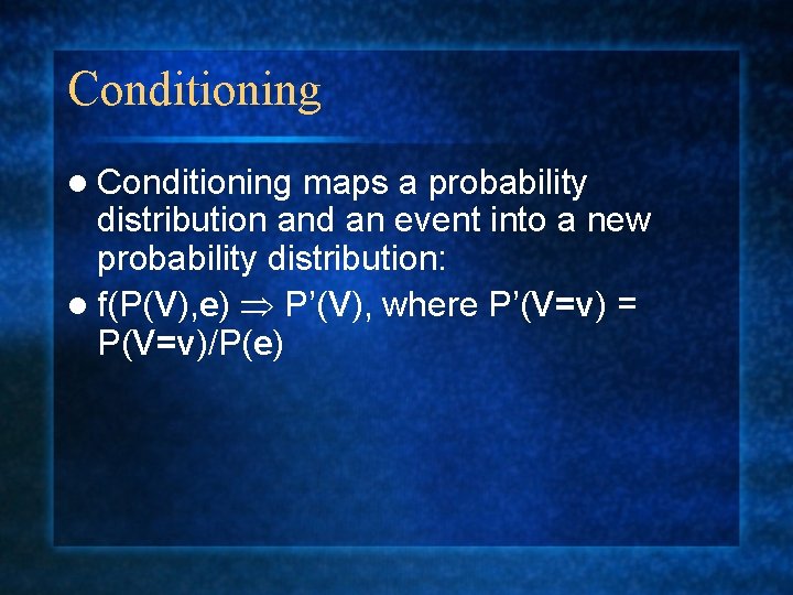
Conditioning l Conditioning maps a probability distribution and an event into a new probability distribution: l f(P(V), e) P’(V), where P’(V=v) = P(V=v)/P(e)

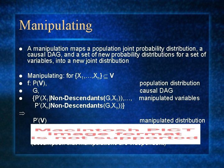
Manipulating l A manipulation maps a population joint probability distribution, a causal DAG, and a set of new probability distributions for a set of variables, into a new joint distribution l l Manipulating: for {X 1, …, Xn} V f: P(V), G, {P’(X 1|Non-Descendants(G, X 1)), …, P’(Xn|Non-Descendants(G, Xn))} P’(V) population distribution causal DAG manipulated variables manipulated distribution (assumption that manipulations are independent)

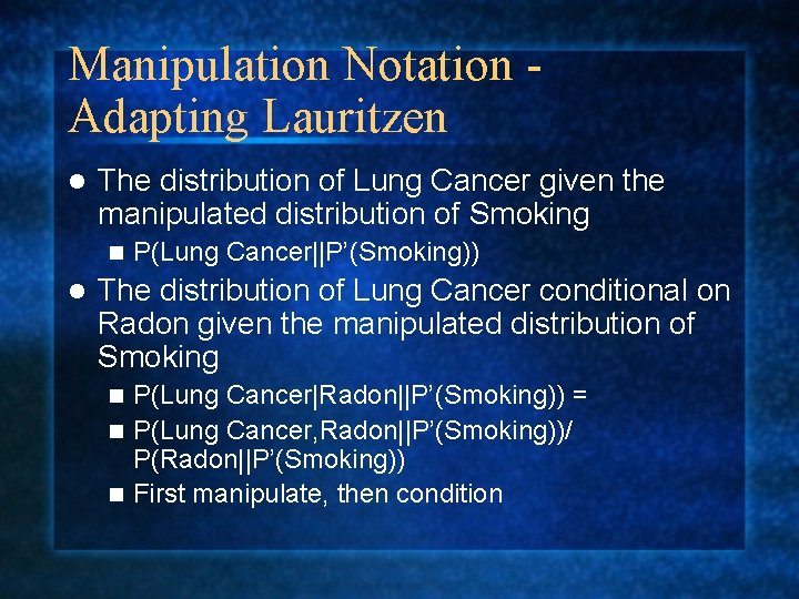
Manipulation Notation Adapting Lauritzen l The distribution of Lung Cancer given the manipulated distribution of Smoking n l P(Lung Cancer||P’(Smoking)) The distribution of Lung Cancer conditional on Radon given the manipulated distribution of Smoking P(Lung Cancer|Radon||P’(Smoking)) = n P(Lung Cancer, Radon||P’(Smoking))/ P(Radon||P’(Smoking)) n First manipulate, then condition n

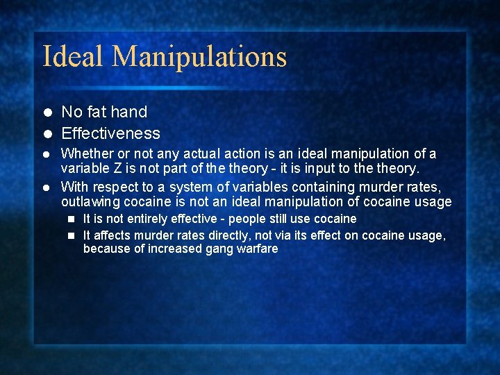
Ideal Manipulations No fat hand l Effectiveness l Whether or not any actual action is an ideal manipulation of a variable Z is not part of theory - it is input to theory. l With respect to a system of variables containing murder rates, outlawing cocaine is not an ideal manipulation of cocaine usage l It is not entirely effective - people still use cocaine n It affects murder rates directly, not via its effect on cocaine usage, because of increased gang warfare n

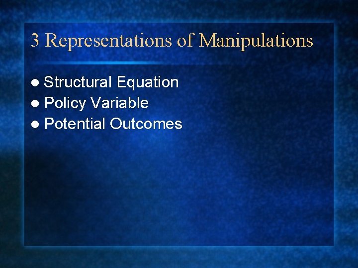
3 Representations of Manipulations l Structural Equation l Policy Variable l Potential Outcomes

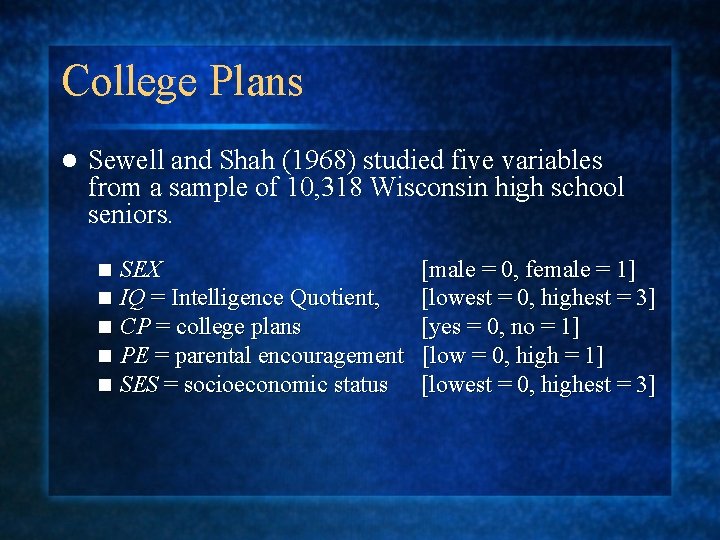
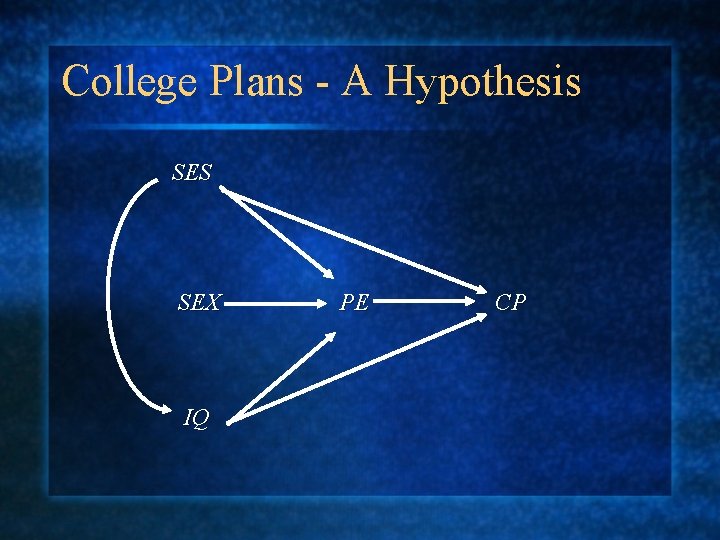
College Plans l Sewell and Shah (1968) studied five variables from a sample of 10, 318 Wisconsin high school seniors. n n n SEX IQ = Intelligence Quotient, CP = college plans PE = parental encouragement SES = socioeconomic status [male = 0, female = 1] [lowest = 0, highest = 3] [yes = 0, no = 1] [low = 0, high = 1] [lowest = 0, highest = 3]

College Plans - A Hypothesis SES SEX IQ PE CP

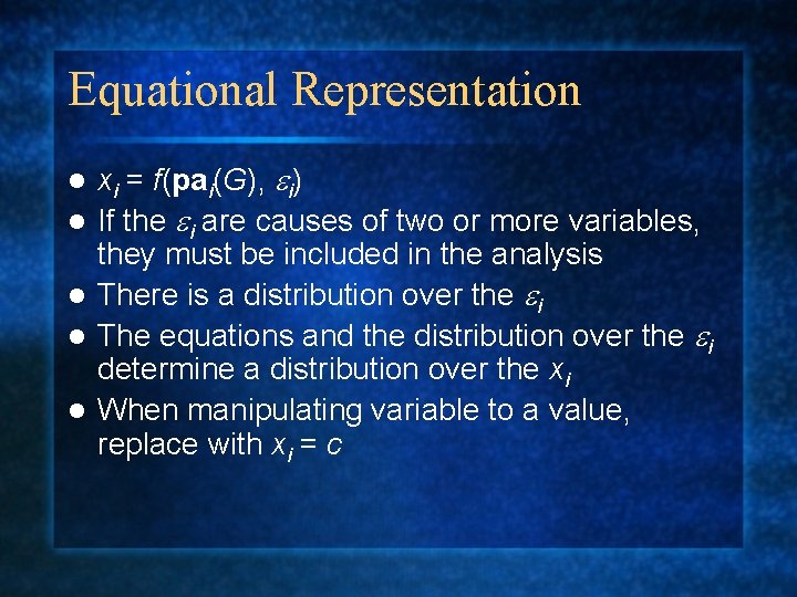
Equational Representation l l l xi = f(pai(G), ei) If the ei are causes of two or more variables, they must be included in the analysis There is a distribution over the ei The equations and the distribution over the ei determine a distribution over the xi When manipulating variable to a value, replace with xi = c

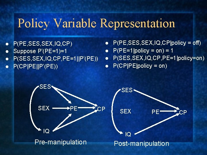
Policy Variable Representation P(PE, SES, SEX, IQ, CP) l Suppose P’(PE=1)=1 l P(SES, SEX, IQ, CP, PE=1||P’(PE)) l P(CP|PE||P’(PE)) l SES SEX P(PE, SES, SEX, IQ, CP|policy = off) l P(PE=1|policy = on) = 1 l P(SES, SEX, IQ, CP, PE=1|policy=on) l P(CP|PE|policy = on) l SES PE IQ Pre-manipulation CP SEX PE IQ Post-manipulation CP

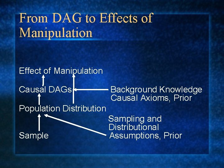
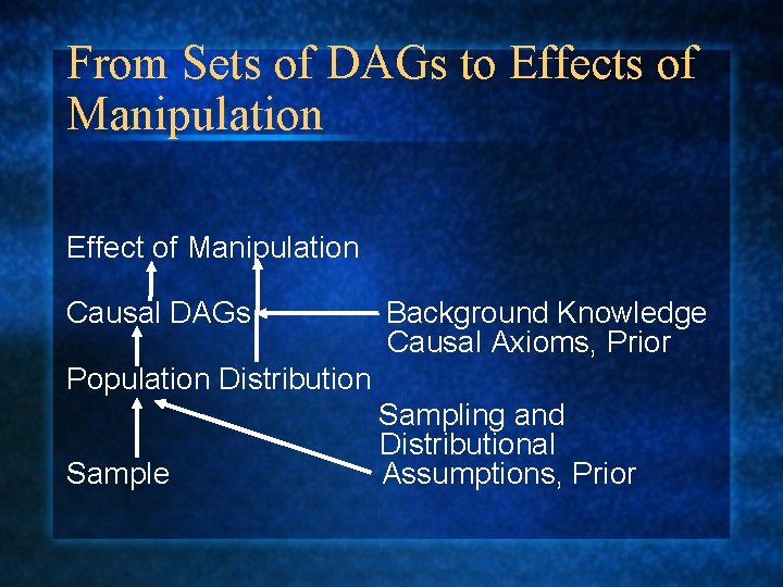
From DAG to Effects of Manipulation Effect of Manipulation Causal DAGs Background Knowledge Causal Axioms, Prior Population Distribution Sample Sampling and Distributional Assumptions, Prior

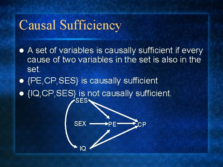
Causal Sufficiency A set of variables is causally sufficient if every cause of two variables in the set is also in the set. l {PE, CP, SES} is causally sufficient l {IQ, CP, SES} is not causally sufficient. l SES SEX IQ PE CP

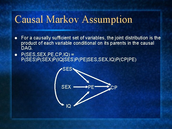
Causal Markov Assumption For a causally sufficient set of variables, the joint distribution is the product of each variable conditional on its parents in the causal DAG. l P(SES, SEX, PE, CP, IQ) = P(SES)P(SEX)P(IQ|SES)P(PE|SES, SEX, IQ)P(CP|PE) l SES SEX IQ PE CP

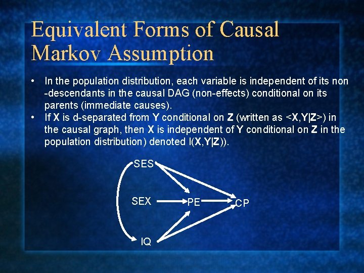
Equivalent Forms of Causal Markov Assumption • In the population distribution, each variable is independent of its non -descendants in the causal DAG (non-effects) conditional on its parents (immediate causes). • If X is d-separated from Y conditional on Z (written as <X, Y|Z>) in the causal graph, then X is independent of Y conditional on Z in the population distribution) denoted I(X, Y|Z)). SES SEX IQ PE CP

Causal Markov Assumption Causal Markov implies that if X is d-separated from Y conditional on Z in the causal DAG, then X is independent of Y conditional on Z. l Causal Markov is equivalent to assuming that the causal DAG represents the population distribution. l What would a failure of Causal Markov look like? If X and Y are dependent, but X does not cause Y, Y does not cause X, and no variable Z causes both X and Y. l

Causal Markov Assumption l Assumes that no unit in the population affects other units in the population If the “natural” units do affect each other, the units should be re-defined to be aggregations of units that don’t affect each other n For example, individual people might be aggregated into families n Assumes variables are not logically related, e. g. x and x 2 l Assumes no feedback l

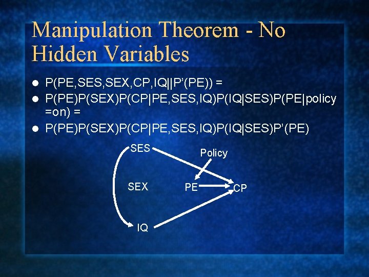
Manipulation Theorem - No Hidden Variables P(PE, SES, SEX, CP, IQ||P’(PE)) = l P(PE)P(SEX)P(CP|PE, SES, IQ)P(IQ|SES)P(PE|policy =on) = l P(PE)P(SEX)P(CP|PE, SES, IQ)P(IQ|SES)P’(PE) l SES SEX IQ Policy PE CP

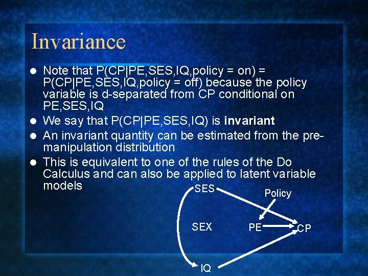
Invariance Note that P(CP|PE, SES, IQ, policy = on) = P(CP|PE, SES, IQ, policy = off) because the policy variable is d-separated from CP conditional on PE, SES, IQ l We say that P(CP|PE, SES, IQ) is invariant l An invariant quantity can be estimated from the premanipulation distribution l This is equivalent to one of the rules of the Do Calculus and can also be applied to latent variable models SES l Policy SEX IQ PE CP

SES Calculating Effects SEX IQ Policy PE CP

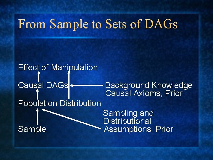
From Sample to Sets of DAGs Effect of Manipulation Causal DAGs Background Knowledge Causal Axioms, Prior Population Distribution Sample Sampling and Distributional Assumptions, Prior

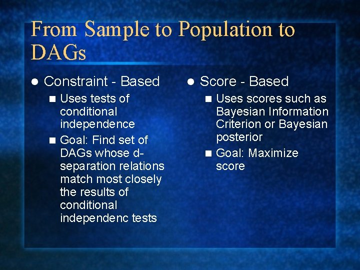
From Sample to Population to DAGs l Constraint - Based Uses tests of conditional independence n Goal: Find set of DAGs whose dseparation relations match most closely the results of conditional independenc tests n l Score - Based Uses scores such as Bayesian Information Criterion or Bayesian posterior n Goal: Maximize score n

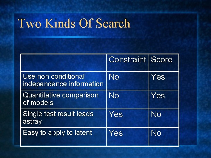
Two Kinds Of Search Constraint Score Use non conditional No independence information Yes Quantitative comparison of models No Yes Single test result leads astray Yes No Easy to apply to latent Yes No

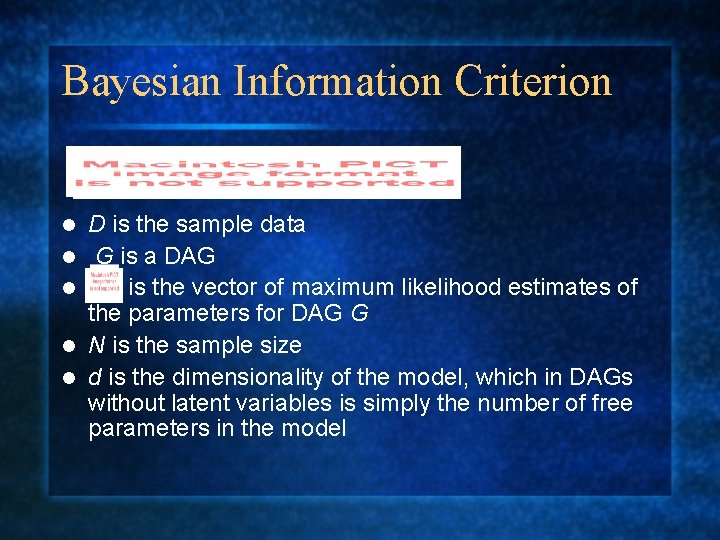
Bayesian Information Criterion l l l D is the sample data G is a DAG is the vector of maximum likelihood estimates of the parameters for DAG G N is the sample size d is the dimensionality of the model, which in DAGs without latent variables is simply the number of free parameters in the model

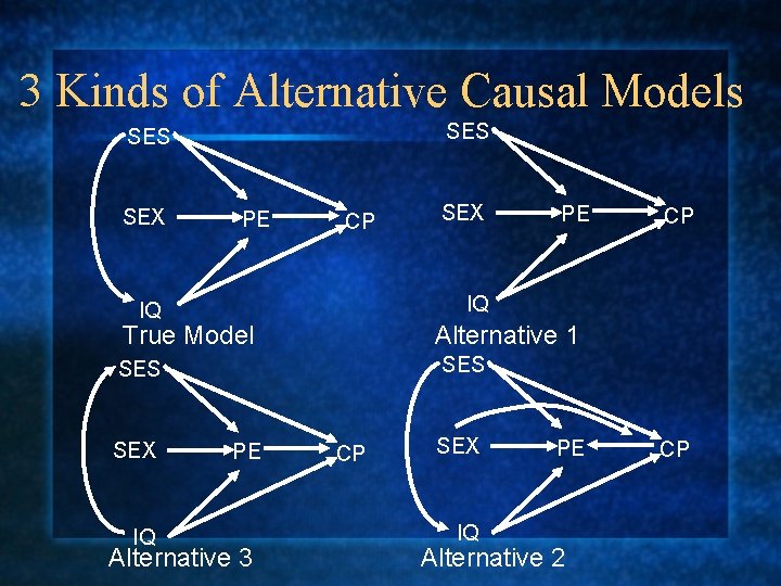
3 Kinds of Alternative Causal Models SES SEX PE CP True Model CP Alternative 1 SES IQ PE IQ IQ SEX PE Alternative 3 CP SEX IQ PE Alternative 2 CP

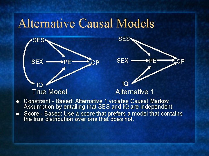
Alternative Causal Models SES SEX IQ PE True Model CP SEX PE CP IQ Alternative 1 Constraint - Based: Alternative 1 violates Causal Markov Assumption by entailing that SES and IQ are independent l Score - Based: Use a score that prefers a model that contains the true distribution over one that does not. l

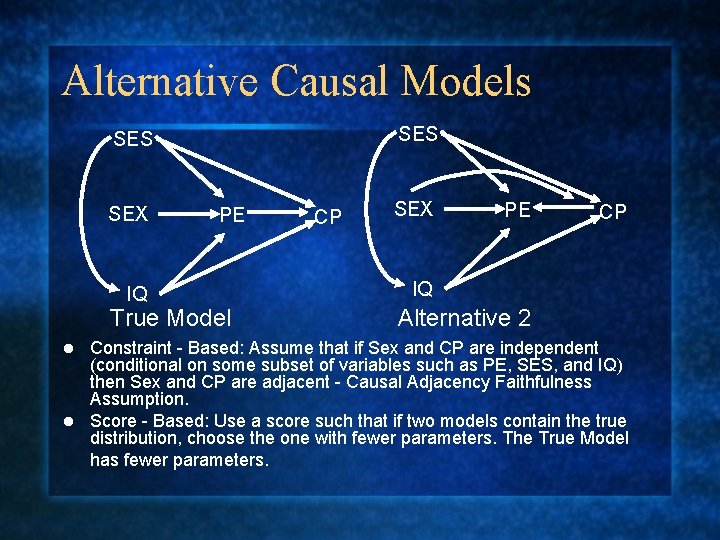
Alternative Causal Models SES SEX IQ PE True Model CP SEX PE CP IQ Alternative 2 Constraint - Based: Assume that if Sex and CP are independent (conditional on some subset of variables such as PE, SES, and IQ) then Sex and CP are adjacent - Causal Adjacency Faithfulness Assumption. l Score - Based: Use a score such that if two models contain the true distribution, choose the one with fewer parameters. The True Model has fewer parameters. l

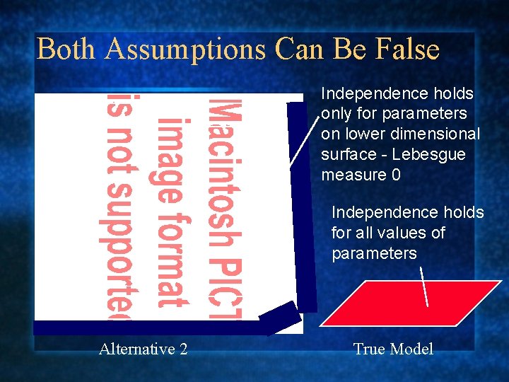
Both Assumptions Can Be False Independence holds only for parameters on lower dimensional surface - Lebesgue measure 0 Independence holds for all values of parameters Alternative 2 True Model

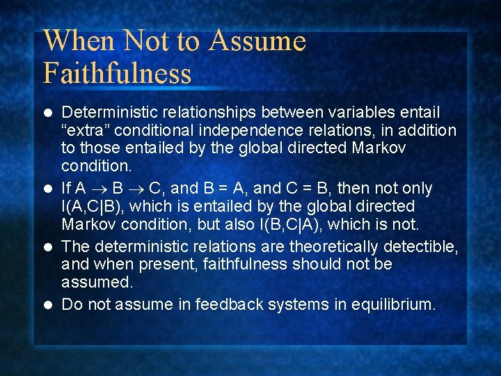
When Not to Assume Faithfulness Deterministic relationships between variables entail “extra” conditional independence relations, in addition to those entailed by the global directed Markov condition. l If A B C, and B = A, and C = B, then not only I(A, C|B), which is entailed by the global directed Markov condition, but also I(B, C|A), which is not. l The deterministic relations are theoretically detectible, and when present, faithfulness should not be assumed. l Do not assume in feedback systems in equilibrium. l

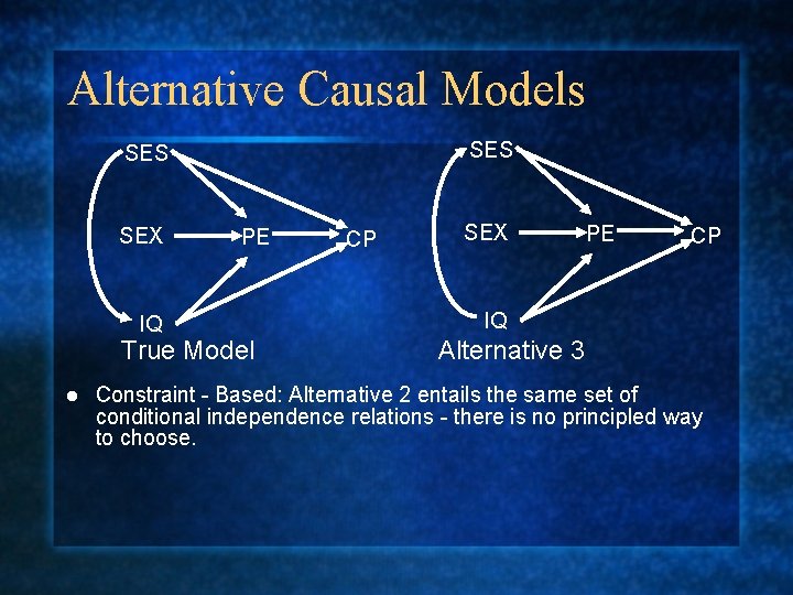
Alternative Causal Models SES SEX IQ PE True Model l CP SEX PE CP IQ Alternative 3 Constraint - Based: Alternative 2 entails the same set of conditional independence relations - there is no principled way to choose.

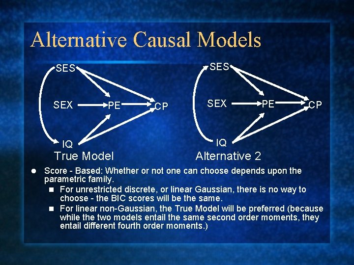
Alternative Causal Models SES SEX IQ PE True Model l CP SEX PE CP IQ Alternative 2 Score - Based: Whether or not one can choose depends upon the parametric family. n For unrestricted discrete, or linear Gaussian, there is no way to choose - the BIC scores will be the same. n For linear non-Gaussian, the True Model will be preferred (because while the two models entail the same second order moments, they entail different fourth order moments. )

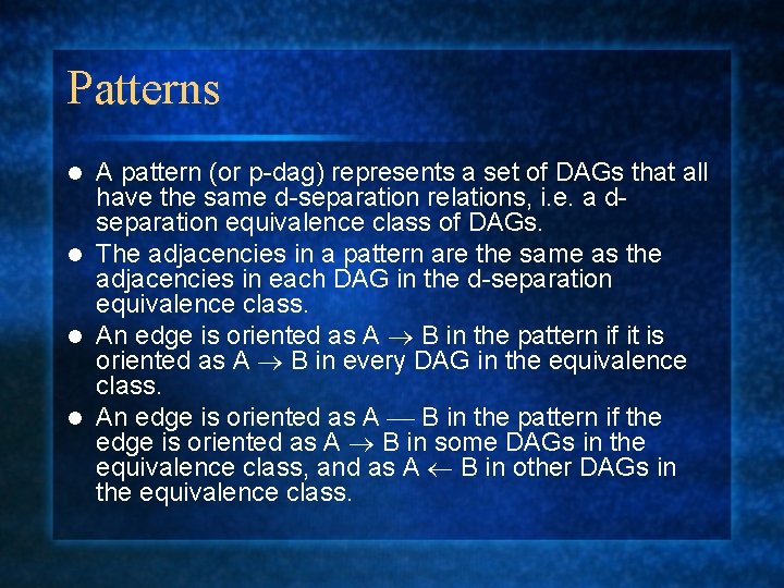
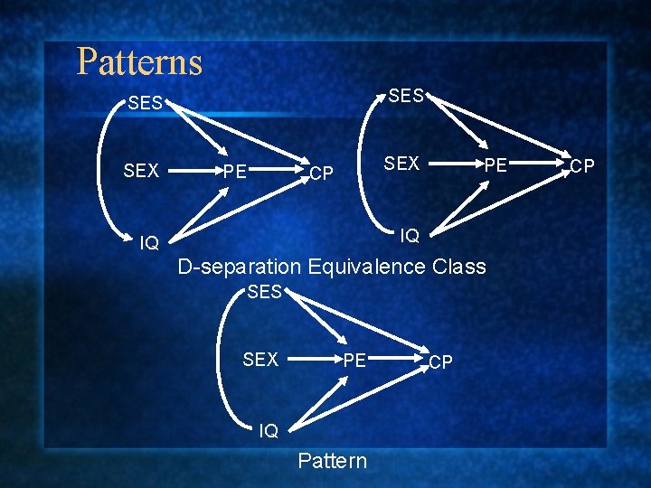
Patterns A pattern (or p-dag) represents a set of DAGs that all have the same d-separation relations, i. e. a dseparation equivalence class of DAGs. l The adjacencies in a pattern are the same as the adjacencies in each DAG in the d-separation equivalence class. l An edge is oriented as A B in the pattern if it is oriented as A B in every DAG in the equivalence class. l An edge is oriented as A B in the pattern if the edge is oriented as A B in some DAGs in the equivalence class, and as A B in other DAGs in the equivalence class. l

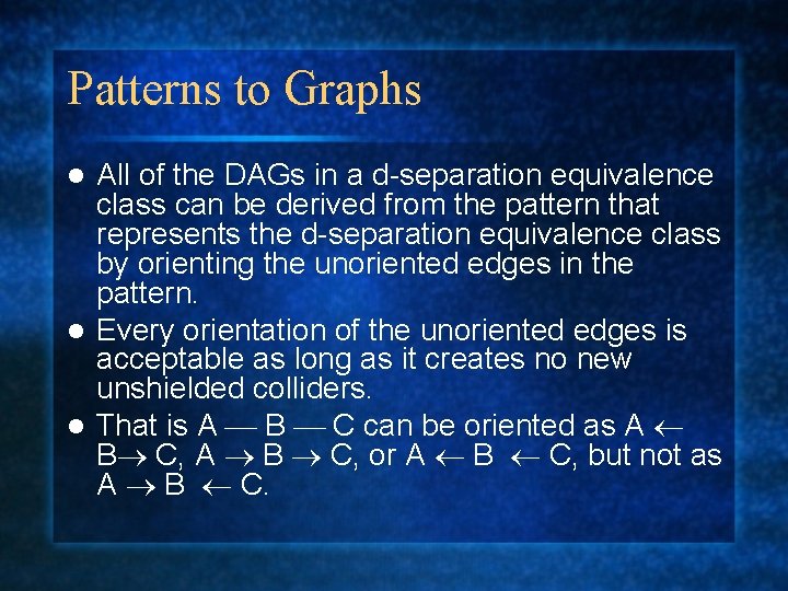
Patterns to Graphs All of the DAGs in a d-separation equivalence class can be derived from the pattern that represents the d-separation equivalence class by orienting the unoriented edges in the pattern. l Every orientation of the unoriented edges is acceptable as long as it creates no new unshielded colliders. l That is A B C can be oriented as A B C, A B C, or A B C, but not as A B C. l

Patterns SES SEX PE SEX CP PE IQ IQ D-separation Equivalence Class SES SEX PE IQ Pattern CP CP

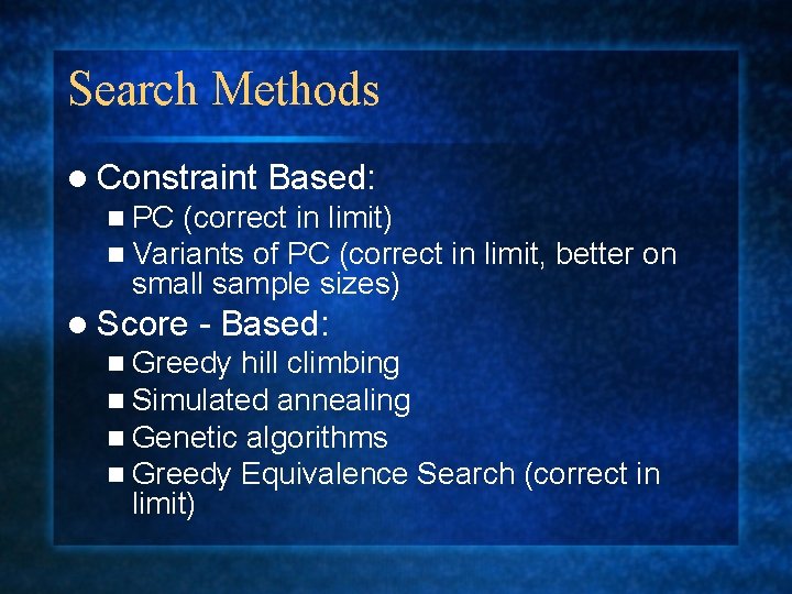
Search Methods l Constraint Based: n PC (correct in limit) n Variants of PC (correct small sample sizes) l Score in limit, better on - Based: n Greedy hill climbing n Simulated annealing n Genetic algorithms n Greedy Equivalence Search limit) (correct in

From Sets of DAGs to Effects of Manipulation Effect of Manipulation Causal DAGs Background Knowledge Causal Axioms, Prior Population Distribution Sample Sampling and Distributional Assumptions, Prior

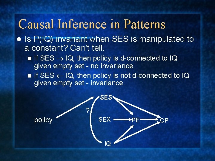
Causal Inference in Patterns l Is P(IQ) invariant when SES is manipulated to a constant? Can’t tell. If SES IQ, then policy is d-connected to IQ given empty set - no invariance. n If SES IQ, then policy is not d-connected to IQ given empty set - invariance. n SES ? policy SEX IQ PE CP

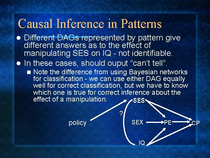
Causal Inference in Patterns Different DAGs represented by pattern give different answers as to the effect of manipulating SES on IQ - not identifiable. l In these cases, should ouput “can’t tell”. l n Note the difference from using Bayesian networks for classification - we can use either DAG equally well for correct classification, but we have to know which one is true for correct inference about the effect of a manipulation. SES ? policy SEX IQ PE CP

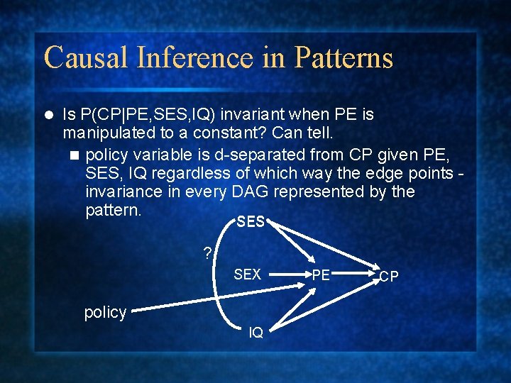
Causal Inference in Patterns l Is P(CP|PE, SES, IQ) invariant when PE is manipulated to a constant? Can tell. n policy variable is d-separated from CP given PE, SES, IQ regardless of which way the edge points invariance in every DAG represented by the pattern. SES ? SEX policy IQ PE CP

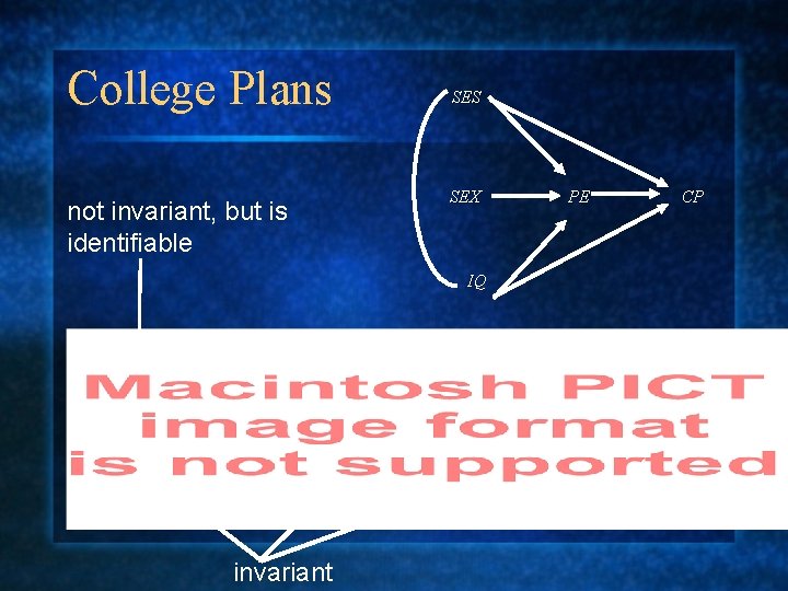
College Plans not invariant, but is identifiable SES SEX IQ invariant PE CP

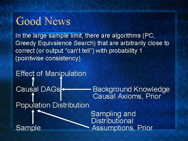
Good News In the large sample limit, there algorithms (PC, Greedy Equivalence Search) that are arbitrarily close to correct (or output “can’t tell”) with probability 1 (pointwise consistency). Effect of Manipulation Causal DAGs Background Knowledge Causal Axioms, Prior Population Distribution Sample Sampling and Distributional Assumptions, Prior

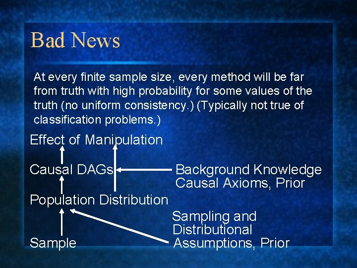
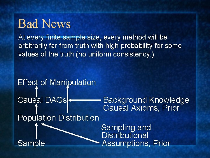
Bad News At every finite sample size, every method will be far from truth with high probability for some values of the truth (no uniform consistency. ) (Typically not true of classification problems. ) Effect of Manipulation Causal DAGs Background Knowledge Causal Axioms, Prior Population Distribution Sample Sampling and Distributional Assumptions, Prior

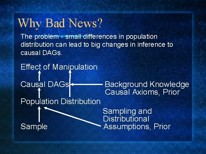
Why Bad News? The problem - small differences in population distribution can lead to big changes in inference to causal DAGs. Effect of Manipulation Causal DAGs Background Knowledge Causal Axioms, Prior Population Distribution Sample Sampling and Distributional Assumptions, Prior

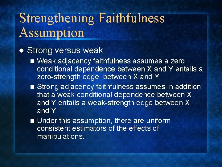
Strengthening Faithfulness Assumption l Strong versus weak Weak adjacency faithfulness assumes a zero conditional dependence between X and Y entails a zero-strength edge between X and Y n Strong adjacency faithfulness assumes in addition that a weak conditional dependence between X and Y entails a weak-strength edge between X and Y n Under this assumption, there are uniform consistent estimators of the effects of manipulations. n

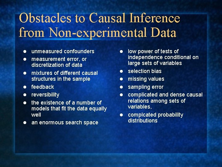
Obstacles to Causal Inference from Non-experimental Data l l l l unmeasured confounders measurement error, or discretization of data mixtures of different causal structures in the sample feedback reversibility the existence of a number of models that fit the data equally well an enormous search space l l l low power of tests of independence conditional on large sets of variables selection bias missing values sampling error complicated and dense causal relations among sets of variables, complcated probability distributions

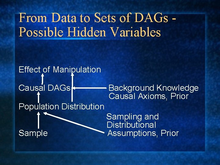
From Data to Sets of DAGs Possible Hidden Variables Effect of Manipulation Causal DAGs Background Knowledge Causal Axioms, Prior Population Distribution Sample Sampling and Distributional Assumptions, Prior

Why Latent Variable Models? l For classification problems, introducing latent variables can help get closer to the right answer at smaller sample sizes - but they are needed to get the right answer in the limit. l For causal inference problems, introducing latent variables are needed to get the right answer in the limit.

Score-Based Search Over Latent Models l Structural EM interleaves estimation of parameters with structural search l Can also search over latent variable models by calculating posteriors l But there are substantial computational and statistical problems with latent variable models

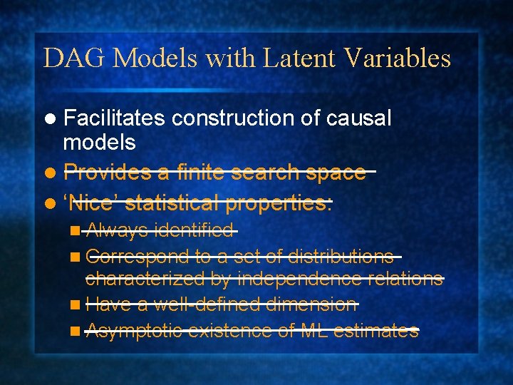
DAG Models with Latent Variables l Facilitates construction of causal models l Provides a finite search space l ‘Nice’ statistical properties: n Always identified n Correspond to a set of distributions characterized by independence relations n Have a well-defined dimension n Asymptotic existence of ML estimates

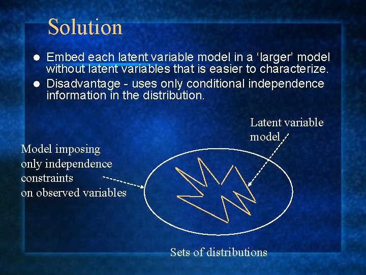
Solution Embed each latent variable model in a ‘larger’ model without latent variables that is easier to characterize. l Disadvantage - uses only conditional independence information in the distribution. l Model imposing only independence constraints on observed variables Latent variable model Sets of distributions

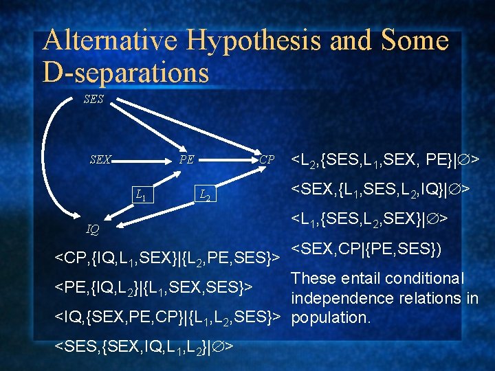
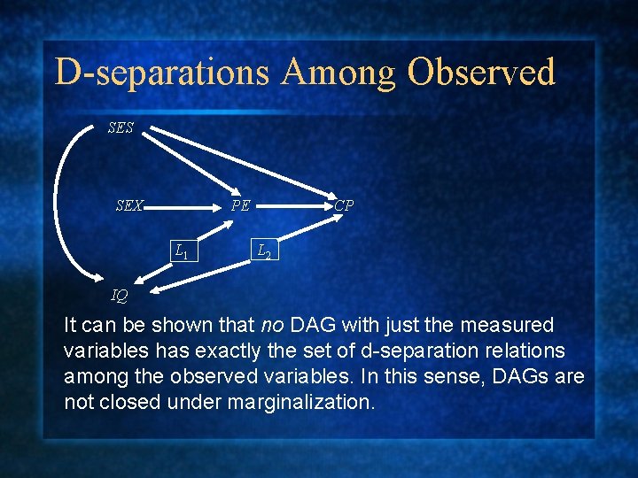
Alternative Hypothesis and Some D-separations SES SEX PE L 1 CP L 2 IQ <CP, {IQ, L 1, SEX}|{L 2, PE, SES}> <L 2, {SES, L 1, SEX, PE}| > <SEX, {L 1, SES, L 2, IQ}| > <L 1, {SES, L 2, SEX}| > <SEX, CP|{PE, SES}) These entail conditional independence relations in <IQ, {SEX, PE, CP}|{L 1, L 2, SES}> population. <PE, {IQ, L 2}|{L 1, SEX, SES}> <SES, {SEX, IQ, L 1, L 2}| >

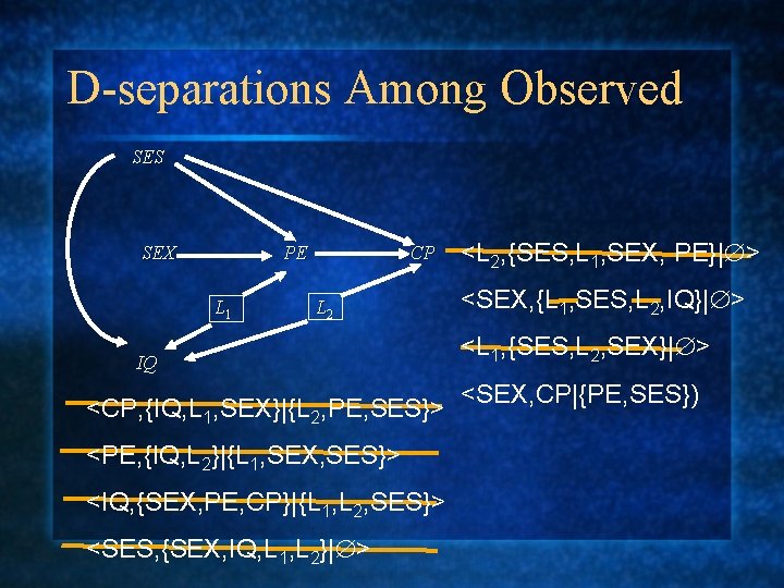
D-separations Among Observed SES SEX PE L 1 CP L 2 IQ <CP, {IQ, L 1, SEX}|{L 2, PE, SES}> <PE, {IQ, L 2}|{L 1, SEX, SES}> <IQ, {SEX, PE, CP}|{L 1, L 2, SES}> <SES, {SEX, IQ, L 1, L 2}| > <L 2, {SES, L 1, SEX, PE}| > <SEX, {L 1, SES, L 2, IQ}| > <L 1, {SES, L 2, SEX}| > <SEX, CP|{PE, SES})

D-separations Among Observed SES SEX PE L 1 CP L 2 IQ It can be shown that no DAG with just the measured variables has exactly the set of d-separation relations among the observed variables. In this sense, DAGs are not closed under marginalization.

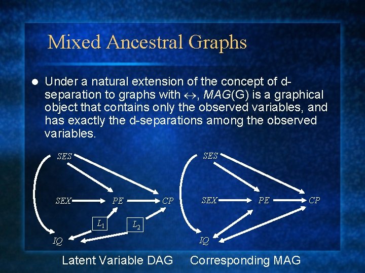
Mixed Ancestral Graphs l Under a natural extension of the concept of dseparation to graphs with , MAG(G) is a graphical object that contains only the observed variables, and has exactly the d-separations among the observed variables. SES SEX PE L 1 CP SEX PE L 2 IQ Latent Variable DAG IQ Corresponding MAG CP

Mixed Ancestral Graph Construction There is an edge between A and B if and only if for every <{A}, {B}|C>, there is a latent variable in C. l If A and B are adjacent, then A B if and only if A is an ancestor of B. l If A and B are adjacent, then A B if and only if A is not an ancestor of B and B is not an ancestor of A. l

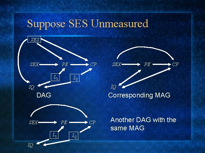
Suppose SES Unmeasured SES SEX PE L 1 CP PE CP L 2 IQ IQ DAG Corresponding MAG SEX PE L 1 IQ SEX CP L 2 Another DAG with the same MAG

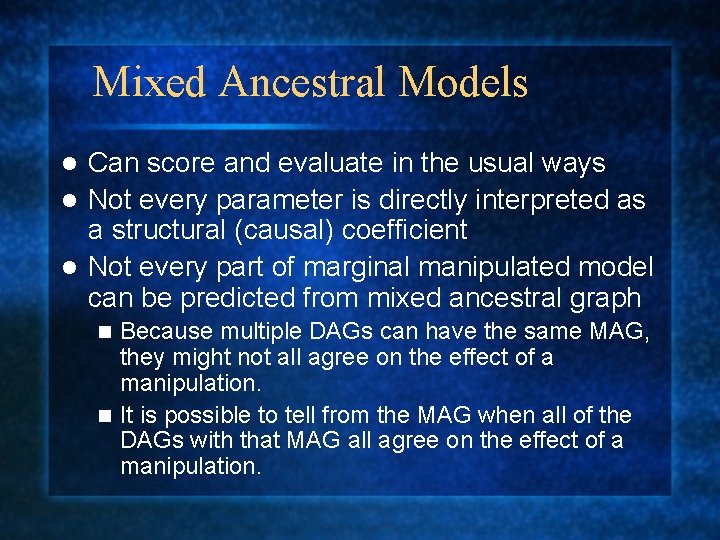
Mixed Ancestral Models Can score and evaluate in the usual ways l Not every parameter is directly interpreted as a structural (causal) coefficient l Not every part of marginal manipulated model can be predicted from mixed ancestral graph l Because multiple DAGs can have the same MAG, they might not all agree on the effect of a manipulation. n It is possible to tell from the MAG when all of the DAGs with that MAG all agree on the effect of a manipulation. n

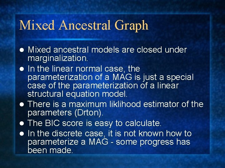
Mixed Ancestral Graph l l l Mixed ancestral models are closed under marginalization. In the linear normal case, the parameterization of a MAG is just a special case of the parameterization of a linear structural equation model. There is a maximum liklihood estimator of the parameters (Drton). The BIC score is easy to calculate. In the discrete case, it is not known how to parameterize a MAG - some progress has been made.

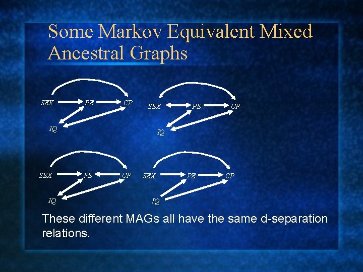
Some Markov Equivalent Mixed Ancestral Graphs SEX PE CP SEX IQ PE CP SEX PE CP IQ These different MAGs all have the same d-separation relations.

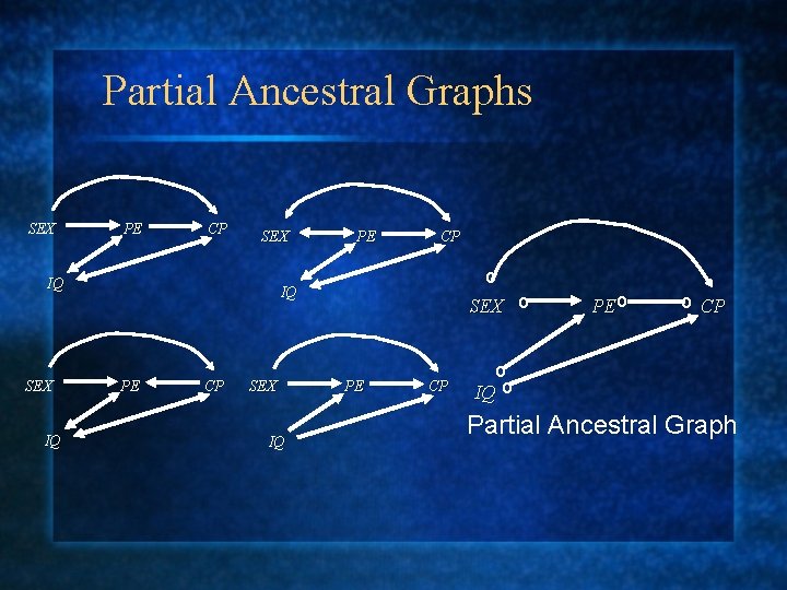
Partial Ancestral Graphs SEX PE CP SEX IQ PE CP o IQ PE CP SEX IQ SEX o PE CP PE o o CP o IQ o Partial Ancestral Graph

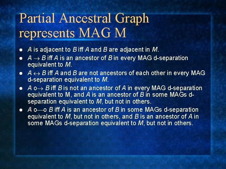
Partial Ancestral Graph represents MAG M l l l A is adjacent to B iff A and B are adjacent in M. A B iff A is an ancestor of B in every MAG d-separation equivalent to M. A B iff A and B are not ancestors of each other in every MAG d-separation equivalent to M. A o B iff B is not an ancestor of A in every MAG d-separation equivalent to M, and A is an ancestor of B in some MAGs dseparation equivalent to M, but not in others. A o o B iff A is an ancestor of B in some MAGs d-separation equivalent to M, but not in others, and B is an ancestor of A in some MAGs d-separation equivalent to M, but not in others.

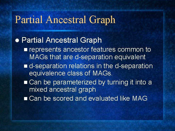
Partial Ancestral Graph l Partial Ancestral Graph n represents ancestor features common to MAGs that are d-separation equivalent n d-separation relations in the d-separation equivalence class of MAGs. n Can be parameterized by turning it into a mixed ancestral graph n Can be scored and evaluated like MAG

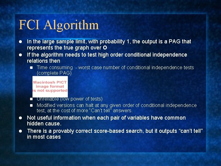
FCI Algorithm In the large sample limit, with probability 1, the output is a PAG that represents the true graph over O l If the algorithm needs to test high order conditional independence relations then l n Time consuming - worst case number of conditional independence tests (complete PAG) Unreliable (low power of tests) n Modified versions can halt at any given order of conditional independence test, at the cost of more “Can’t tell” answers. n Not useful information when each pair of variables have common hidden cause. l There is a provably correct score-based search, but it outputs “can’t tell” in most cases l

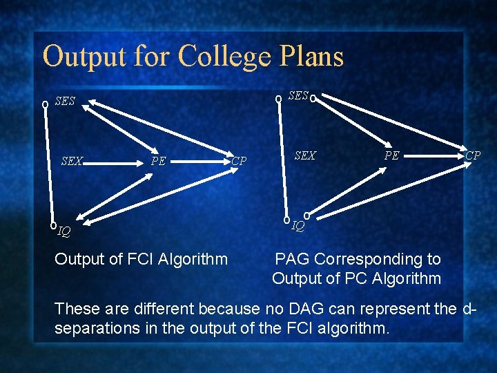
Output for College Plans o SES o o SES SEX PE o. IQ Output of FCI Algorithm CP SEX PE CP o. IQo PAG Corresponding to Output of PC Algorithm These are different because no DAG can represent the dseparations in the output of the FCI algorithm.

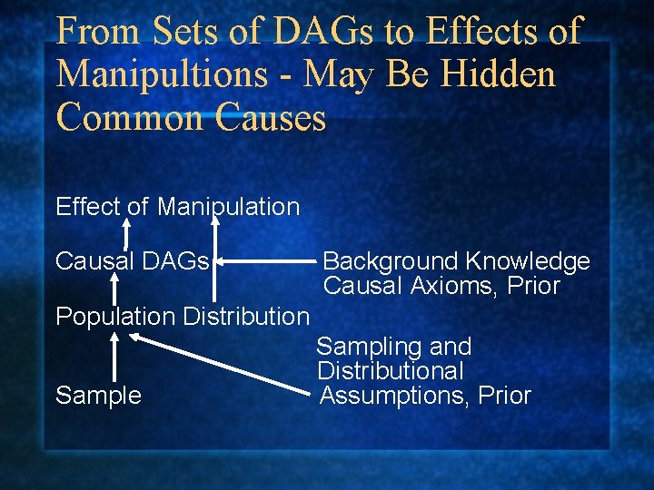
From Sets of DAGs to Effects of Manipultions - May Be Hidden Common Causes Effect of Manipulation Causal DAGs Background Knowledge Causal Axioms, Prior Population Distribution Sample Sampling and Distributional Assumptions, Prior

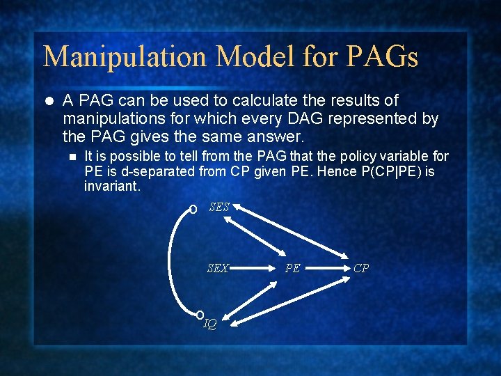
Manipulation Model for PAGs l A PAG can be used to calculate the results of manipulations for which every DAG represented by the PAG gives the same answer. n It is possible to tell from the PAG that the policy variable for PE is d-separated from CP given PE. Hence P(CP|PE) is invariant. o SES SEX o. IQ PE CP

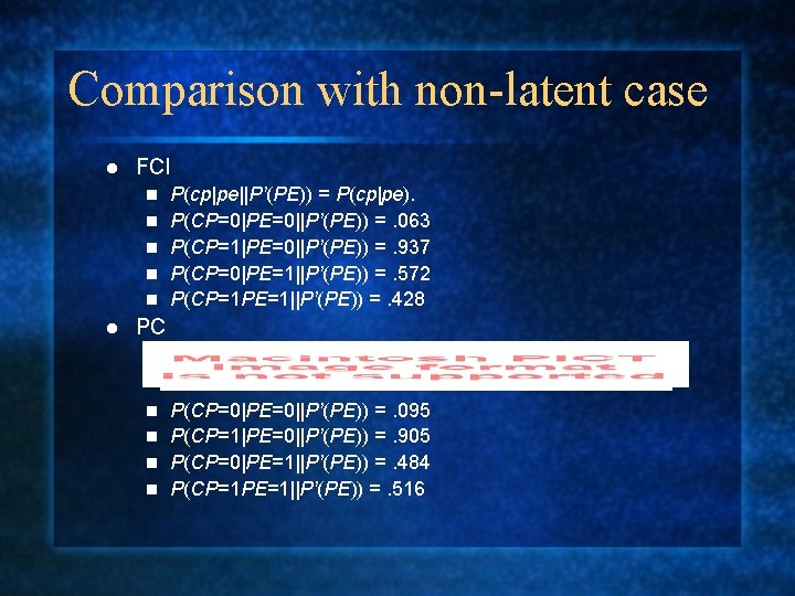
Comparison with non-latent case l FCI n n n l P(cp|pe||P’(PE)) = P(cp|pe). P(CP=0|PE=0||P’(PE)) =. 063 P(CP=1|PE=0||P’(PE)) =. 937 P(CP=0|PE=1||P’(PE)) =. 572 P(CP=1 PE=1||P’(PE)) =. 428 PC P(CP=0|PE=0||P’(PE)) =. 095 n P(CP=1|PE=0||P’(PE)) =. 905 n P(CP=0|PE=1||P’(PE)) =. 484 n P(CP=1 PE=1||P’(PE)) =. 516 n

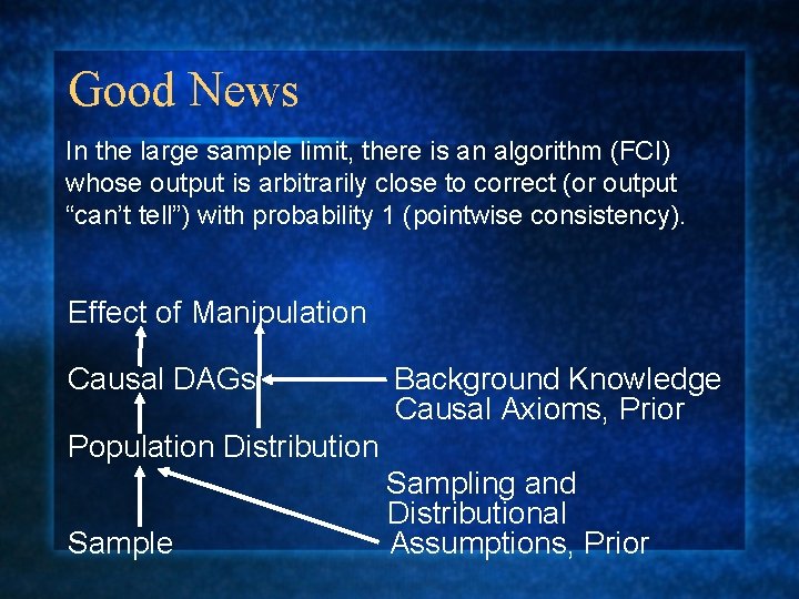
Good News In the large sample limit, there is an algorithm (FCI) whose output is arbitrarily close to correct (or output “can’t tell”) with probability 1 (pointwise consistency). Effect of Manipulation Causal DAGs Background Knowledge Causal Axioms, Prior Population Distribution Sample Sampling and Distributional Assumptions, Prior

Bad News At every finite sample size, every method will be arbitrarily far from truth with high probability for some values of the truth (no uniform consistency. ) Effect of Manipulation Causal DAGs Background Knowledge Causal Axioms, Prior Population Distribution Sample Sampling and Distributional Assumptions, Prior

Other Constraints The disadvantage of using MAGs or FCI is they only use conditional independence information l In the case of latent variable models, there are constraints implied on the observed margin that are not conditional independence relations, regardless of the family of distributions n These can be used to choose between two different latent variable models that have the same d-separation relations over the observed variables l In addition, there are constraints implied on the observed margin that are particular to a family of distributions l

Examples of Open Questions l l l l Complete non-parametric manipulation calculations for partially known DAGs with latent variables Define strong faithfulness for the latent case. Calculating constraints (non-parametric or parametric) from latent variable DAGs Using constraints (non-parametric or parametric) to guide search for latent variable DAGs Latent variable score-based search over PAGs Parameterizations of MAGs for other families of distsributions Completeness of do-calculus for PAGs Time series inference

Introductory Books on Graphical Causal Inference l Causation, Prediction, and Search, by P. Spirtes, C. Glymour, R. Scheines, MIT Press, 2000. l Causality: Models, Reasoning, and Inference by J. Pearl, Cambridge University Press, 2000. l Computation, Causation, and Discovery (Paperback) , ed. by C. Glymour and G. Cooper, AAAI Press, 1999.