Adversarial Search Adversarial Search Game playing Perfect play

Adversarial Search

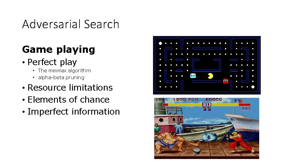
Adversarial Search Game playing • Perfect play • The minimax algorithm • alpha-beta pruning • Resource limitations • Elements of chance • Imperfect information

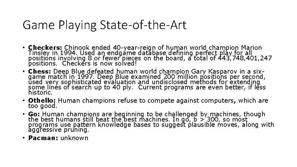
Game Playing State-of-the-Art • Checkers: Chinook ended 40 -year-reign of human world champion Marion Tinsley in 1994. Used an endgame database defining perfect play for all positions involving 8 or fewer pieces on the board, a total of 443, 748, 401, 247 positions. Checkers is now solved! • Chess: Deep Blue defeated human world champion Gary Kasparov in a sixgame match in 1997. Deep Blue examined 200 million positions per second, used very sophisticated evaluation and undisclosed methods for extending some lines of search up to 40 ply. Current programs are even better, if less historic. • Othello: Human champions refuse to compete against computers, which are too good. • Go: Human champions are beginning to be challenged by machines, though the best humans still beat the best machines. In go, b > 300, so most programs use pattern knowledge bases to suggest plausible moves, along with aggressive pruning. • Pacman: unknown

What kind of games? • Abstraction: To describe a game we must capture every relevant aspect of the game. Such as: • Chess • Tic-tac-toe • … • Accessible environments: Such games are characterized by perfect information • Search: game-playing then consists of a search through possible game positions • Unpredictable opponent: introduces uncertainty thus game-playing must deal with contingency problems

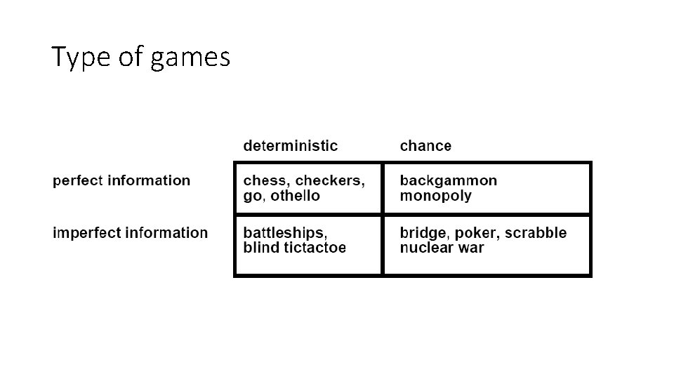
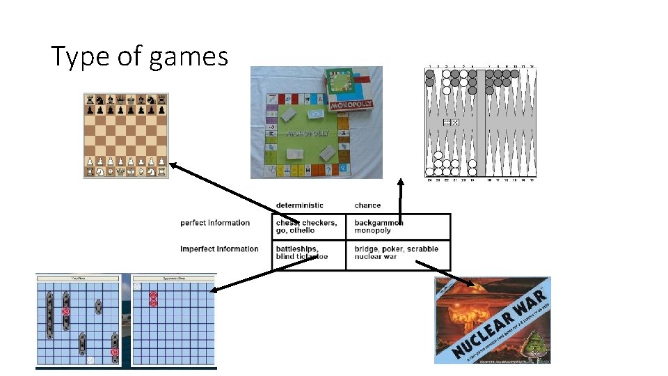
Type of games

Type of games

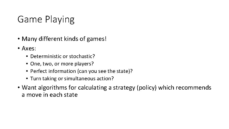
Game Playing • Many different kinds of games! • Axes: • • Deterministic or stochastic? One, two, or more players? Perfect information (can you see the state)? Turn taking or simultaneous action? • Want algorithms for calculating a strategy (policy) which recommends a move in each state

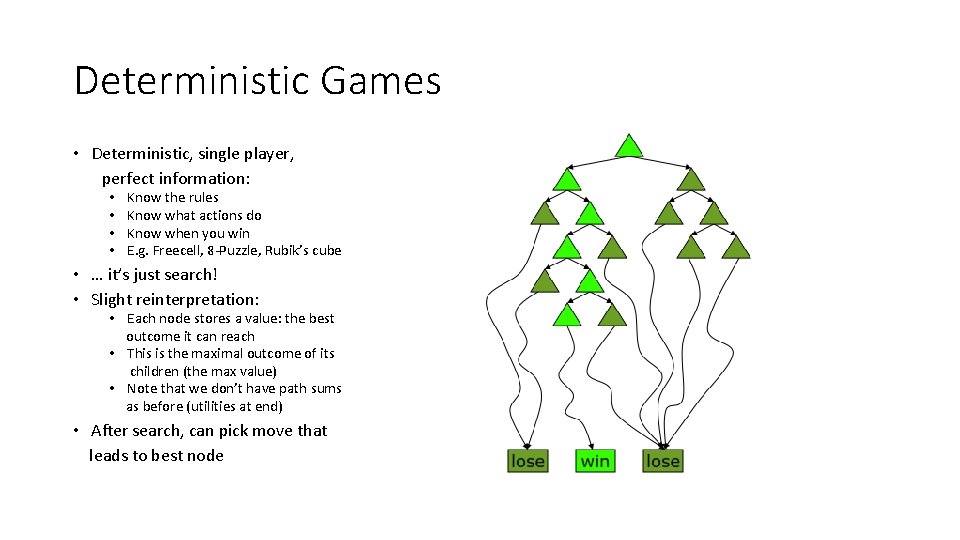
Deterministic Games • Deterministic, single player, perfect information: • • Know the rules Know what actions do Know when you win E. g. Freecell, 8 -Puzzle, Rubik’s cube • … it’s just search! • Slight reinterpretation: • Each node stores a value: the best outcome it can reach • This is the maximal outcome of its children (the max value) • Note that we don’t have path sums as before (utilities at end) • After search, can pick move that leads to best node

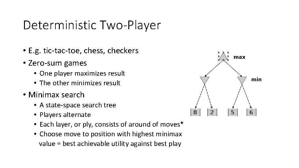
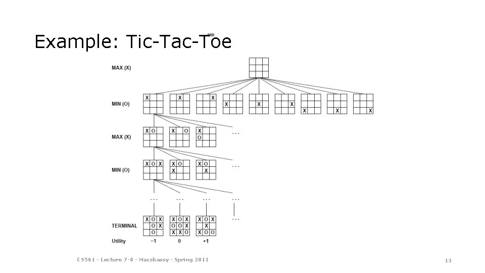
Deterministic Two-Player • E. g. tic-tac-toe, chess, checkers • Zero-sum games • One player maximizes result • The other minimizes result • Minimax search • • A state-space search tree Players alternate Each layer, or ply, consists of around of moves* Choose move to position with highest minimax value = best achievable utility against best play

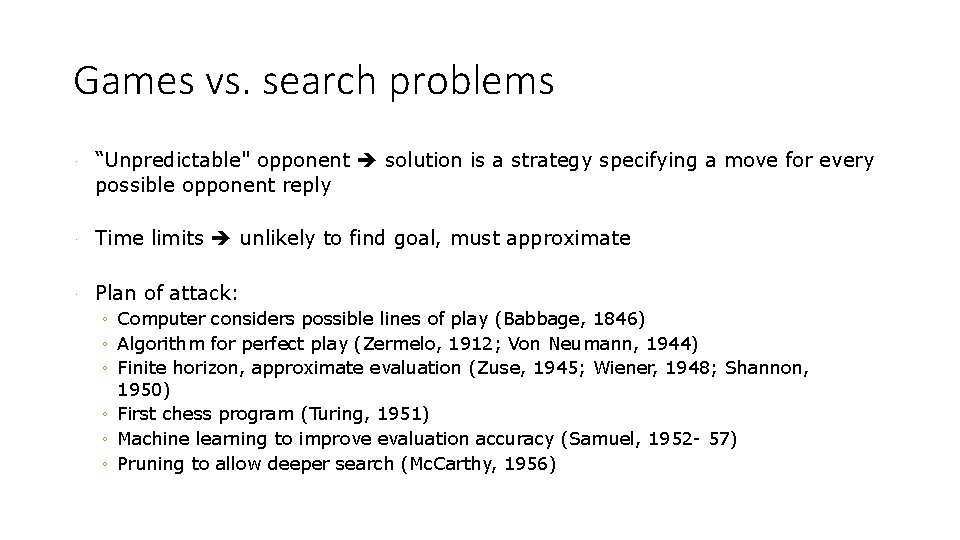
Games vs. search problems · “Unpredictable" opponent solution is a strategy specifying a move for every possible opponent reply · Time limits unlikely to find goal, must approximate · Plan of attack: ◦ Computer considers possible lines of play (Babbage, 1846) ◦ Algorithm for perfect play (Zermelo, 1912; Von Neumann, 1944) ◦ Finite horizon, approximate evaluation (Zuse, 1945; Wiener, 1948; Shannon, 1950) ◦ First chess program (Turing, 1951) ◦ Machine learning to improve evaluation accuracy (Samuel, 1952 - 57) ◦ Pruning to allow deeper search (Mc. Carthy, 1956)

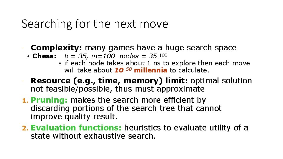
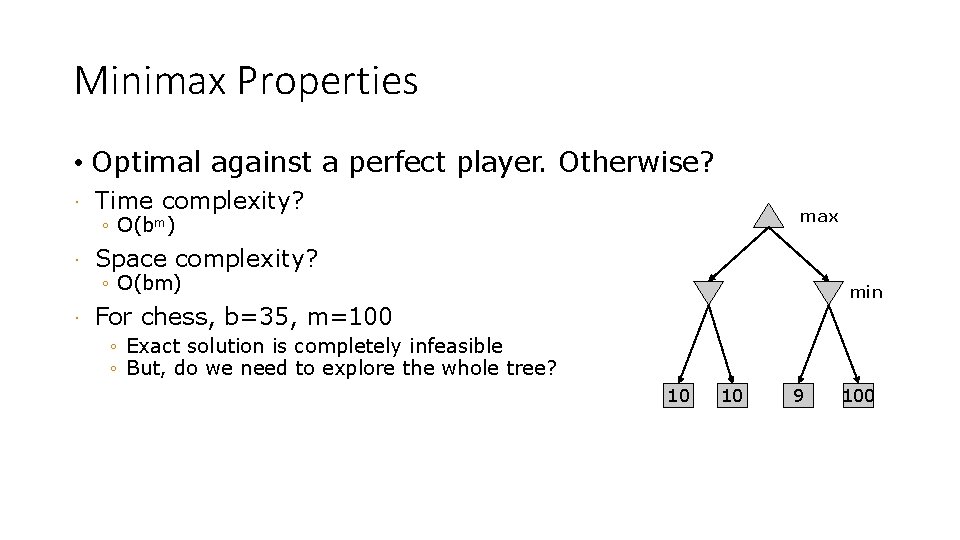
Searching for the next move · Complexity: many games have a huge search space • Chess: b = 35, m=100 nodes = 35 100 • if each node takes about 1 ns to explore then each move will take about 10 50 millennia to calculate. Resource (e. g. , time, memory) limit: optimal solution not feasible/possible, thus must approximate 1. Pruning: makes the search more efficient by discarding portions of the search tree that cannot improve quality result. 2. Evaluation functions: heuristics to evaluate utility of a state without exhaustive search. ·

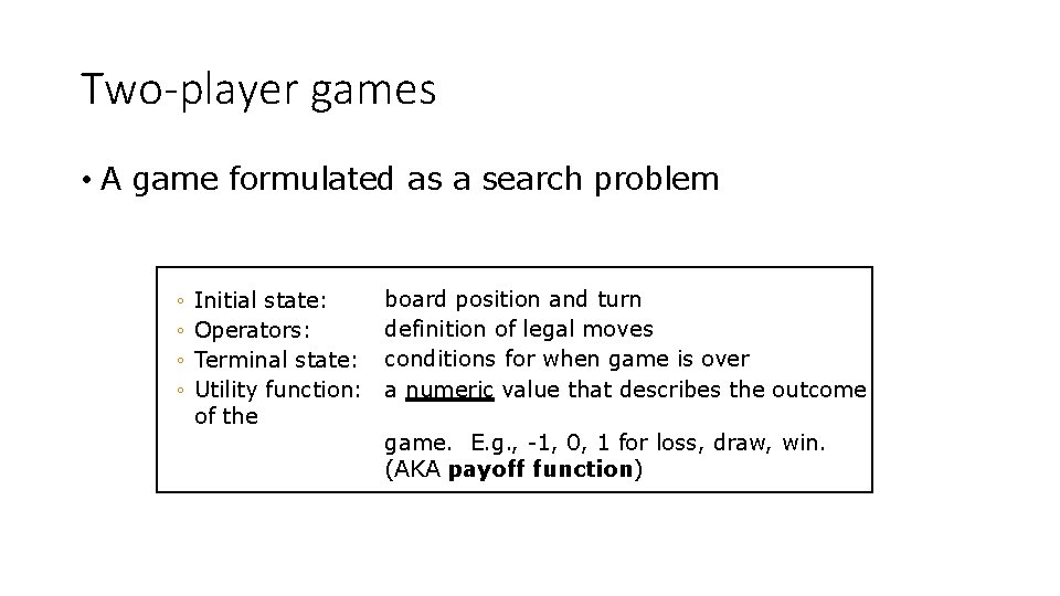
Two-player games • A game formulated as a search problem ◦ ◦ Initial state: Operators: Terminal state: Utility function: of the board position and turn definition of legal moves conditions for when game is over a numeric value that describes the outcome game. E. g. , -1, 0, 1 for loss, draw, win. (AKA payoff function)

Example: Tic-Tac-Toe CS 561 - Lecture 7 -8 - Macskassy - Spring 2011 13

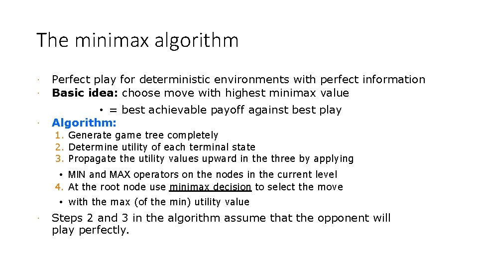
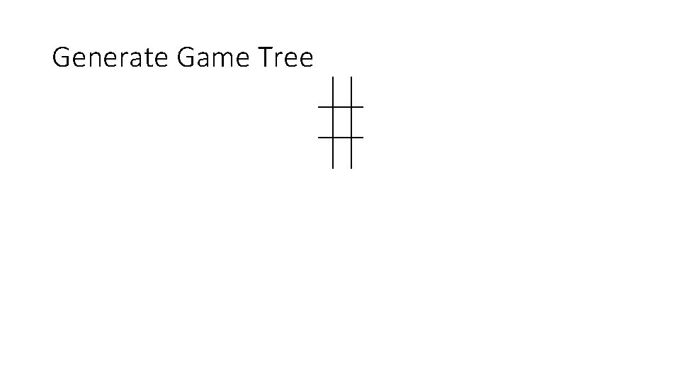
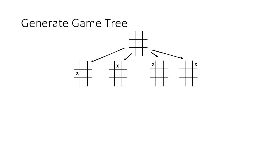
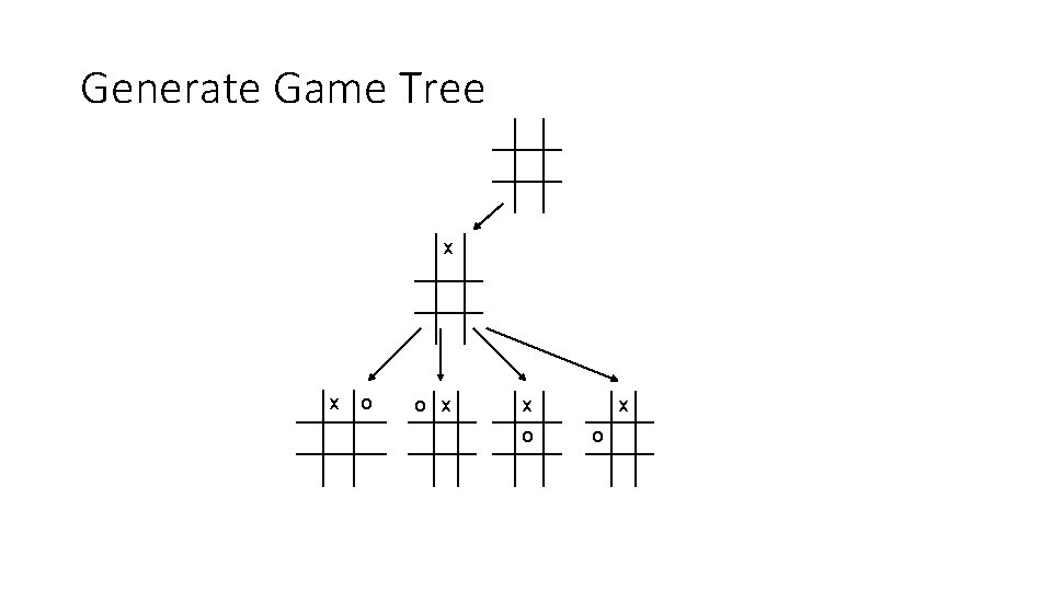
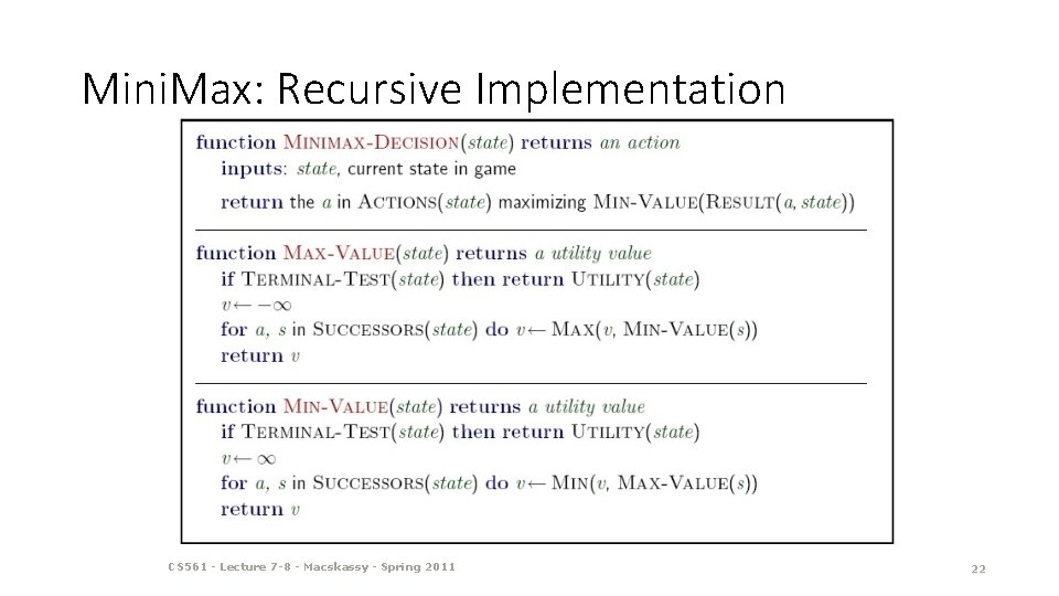
The minimax algorithm · · Perfect play for deterministic environments with perfect information Basic idea: choose move with highest minimax value · • = best achievable payoff against best play Algorithm: 1. Generate game tree completely 2. Determine utility of each terminal state 3. Propagate the utility values upward in the three by applying • MIN and MAX operators on the nodes in the current level 4. At the root node use minimax decision to select the move • with the max (of the min) utility value · Steps 2 and 3 in the algorithm assume that the opponent will play perfectly.

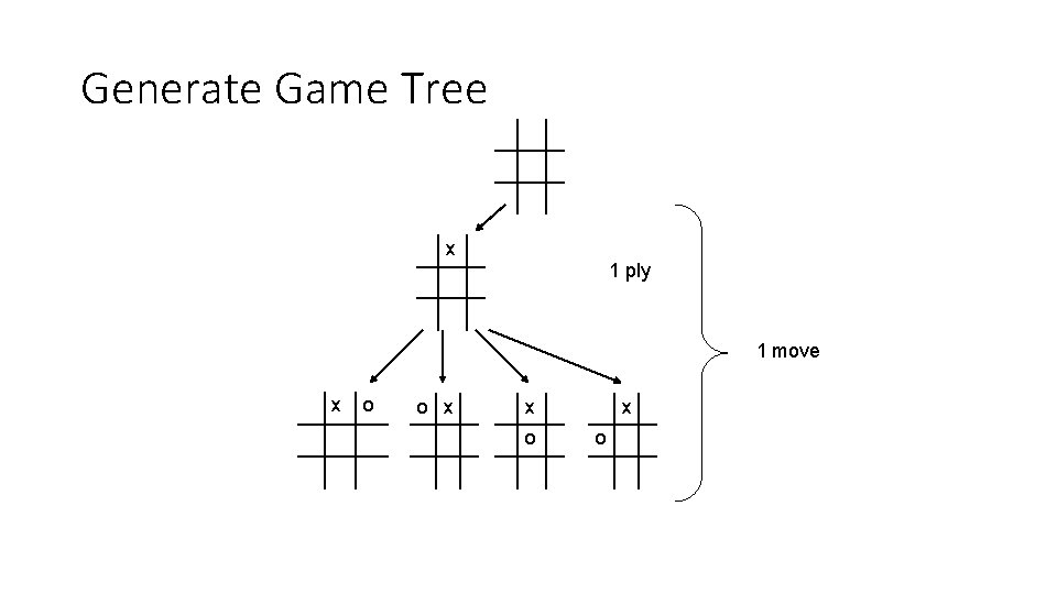
Generate Game Tree

Generate Game Tree x x

Generate Game Tree x x o o x x o

Generate Game Tree x 1 ply 1 move x o o x x o

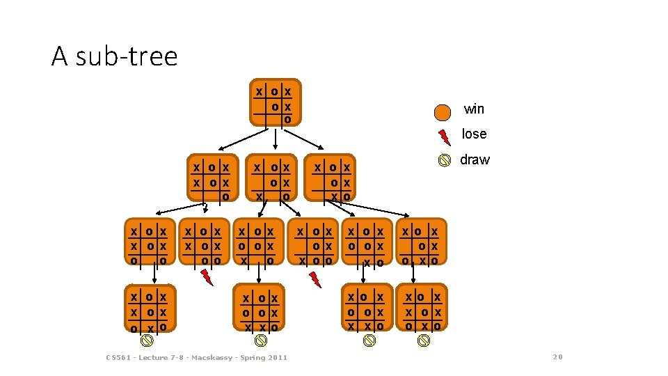
A sub-tree x ox o win lose x o x x ox o x o x x ox oo x ox ox x o x ox o ox x xo CS 561 - Lecture 7 -8 - Macskassy - Spring 2011 draw x o x ox ox x oo x o ox x o x ox o xo x o ox x x ox o 20

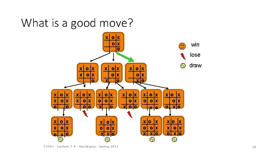
What is a good move? x ox o win lose x o x x ox o x o x x ox oo x ox ox x o x ox o ox x xo CS 561 - Lecture 7 -8 - Macskassy - Spring 2011 draw x o x ox ox x oo x o ox x o x ox o xo x o ox x x ox o 20

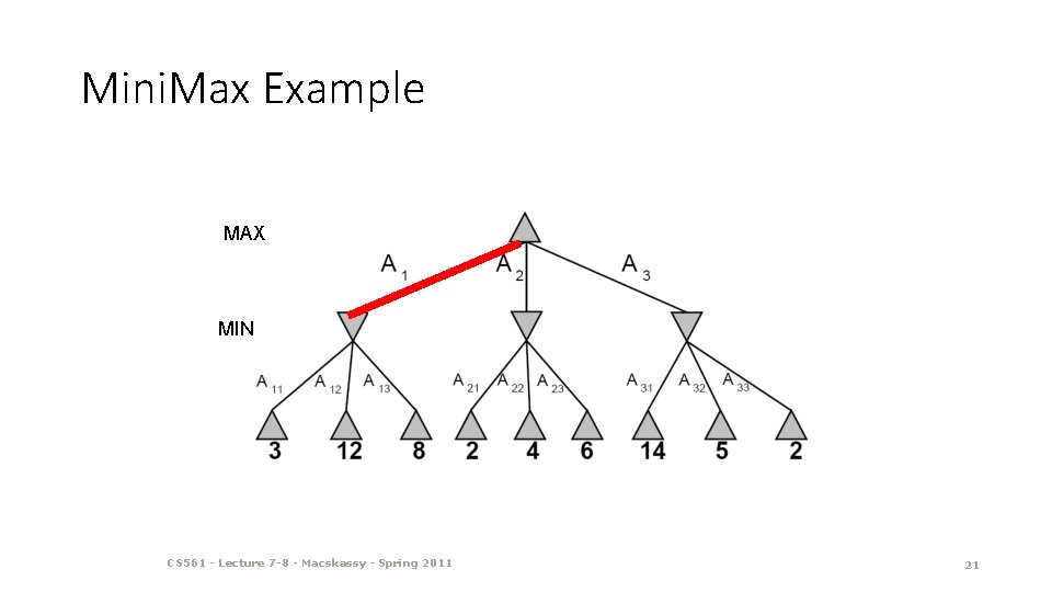
Mini. Max Example MAX MIN CS 561 - Lecture 7 -8 - Macskassy - Spring 2011 21

Mini. Max: Recursive Implementation CS 561 - Lecture 7 -8 - Macskassy - Spring 2011 22

Minimax Properties • Optimal against a perfect player. Otherwise? · Time complexity? · Space complexity? · max ◦ O(bm) min For chess, b=35, m=100 ◦ Exact solution is completely infeasible ◦ But, do we need to explore the whole tree? 10 10 9 100

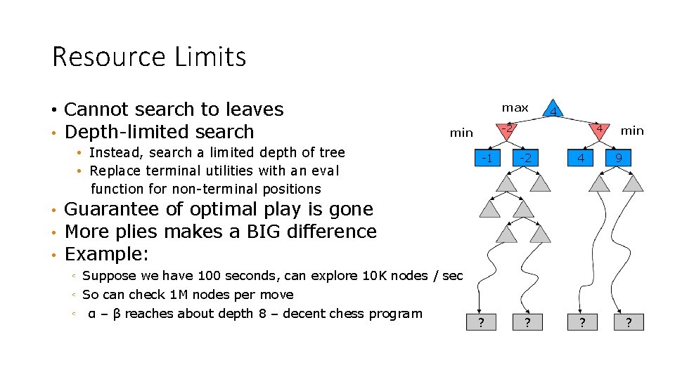
Resource Limits • Cannot search to leaves • Depth-limited search max • • • -2 min • Instead, search a limited depth of tree • Replace terminal utilities with an eval function for non-terminal positions 4 -1 4 -2 4 ? ? min 9 Guarantee of optimal play is gone More plies makes a BIG difference Example: ◦ Suppose we have 100 seconds, can explore 10 K nodes / sec ◦ So can check 1 M nodes per move ◦ α – β reaches about depth 8 – decent chess program ? ?

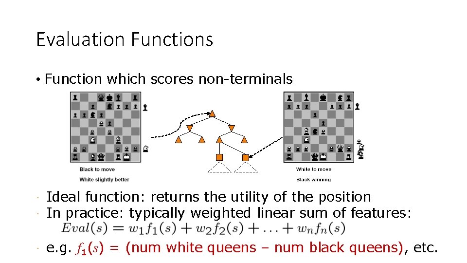
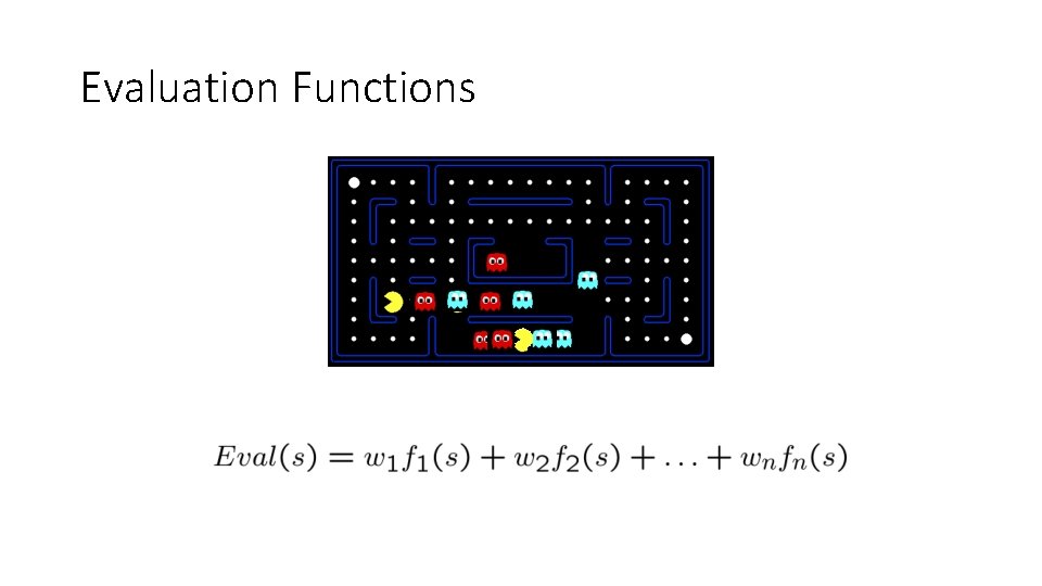
Evaluation Functions • Function which scores non-terminals · · Ideal function: returns the utility of the position In practice: typically weighted linear sum of features: · e. g. f 1(s) = (num white queens – num black queens), etc.

Evaluation Functions

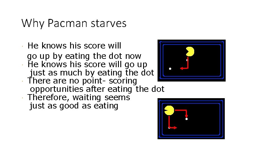
Why Pacman starves He knows his score will go up by eating the dot now · He knows his score will go up just as much by eating the dot later on · There are no point- scoring opportunities after eating the dot · Therefore, waiting seems just as good as eating ·

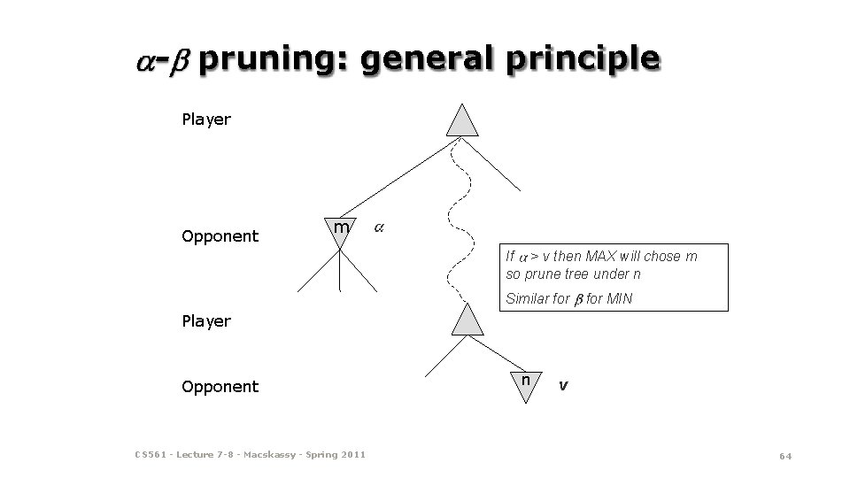
- pruning: general principle Player Opponent m If > v then MAX will chose m so prune tree under n Similar for MIN Player Opponent CS 561 - Lecture 7 -8 - Macskassy - Spring 2011 n v 28

- pruning: example 1 MAX [-∞, +∞] MIN CS 561 - Lecture 7 -8 - Macskassy - Spring 2011 30

- pruning: example 1 [-∞, +∞] MAX MIN 3 CS 561 - Lecture 7 -8 - Macskassy - Spring 2011 30

- pruning: example 1 [-∞, +∞] MAX MIN [-∞, 3] 3 CS 561 - Lecture 7 -8 - Macskassy - Spring 2011 31

- pruning: example 1 [-∞, +∞] MAX MIN [-∞, 3] 3 12 CS 561 - Lecture 7 -8 - Macskassy - Spring 2011 32

- pruning: example 1 [-∞, +∞] [3, +∞] MAX MIN [-∞, 3] 3 12 8 CS 561 - Lecture 7 -8 - Macskassy - Spring 2011 33

- pruning: example 1 [-∞, +∞] [3, +∞] MAX MIN [3, 2] [-∞, 3] 3 12 8 2 CS 561 - Lecture 7 -8 - Macskassy - Spring 2011 34

- pruning: example 1 [-∞, +∞] [3, +∞] MAX MIN [3, 2] [-∞, 3] 3 12 8 2 [3, 14] 14 CS 561 - Lecture 7 -8 - Macskassy - Spring 2011 35

- pruning: example 1 [-∞, +∞] [3, +∞] MAX MIN [3, 2] [-∞, 3] 3 12 8 2 [3, 14] [3, 5] 14 CS 561 - Lecture 7 -8 - Macskassy - Spring 2011 5 36

- pruning: example 1 [-∞, +∞] [3, +∞] MAX MIN [3, 2] [-∞, 3] 3 12 8 2 [3, 14] [3, 5] [3, 2] 14 CS 561 - Lecture 7 -8 - Macskassy - Spring 2011 5 2 37

- pruning: example 1 [-∞, +∞] [3, +∞] MAX Selected move MIN [3, 2] [-∞, 3] 3 12 8 2 [3, 14] [3, 5] [3, 2] 14 CS 561 - Lecture 7 -8 - Macskassy - Spring 2011 5 2 38

- pruning: example 2 MAX [-∞, +∞] MIN CS 561 - Lecture 7 -8 - Macskassy - Spring 2011 40

- pruning: example 2 MAX [-∞, +∞] [-∞, 2] MIN 2 CS 561 - Lecture 7 -8 - Macskassy - Spring 2011 40

- pruning: example 2 MAX [-∞, +∞] [-∞, 2] MIN 5 CS 561 - Lecture 7 -8 - Macskassy - Spring 2011 2 41

- pruning: example 2 MAX [-∞, +∞] [2, +∞] [-∞, 2] MIN 14 CS 561 - Lecture 7 -8 - Macskassy - Spring 2011 5 2 42

- pruning: example 2 MAX [-∞, +∞] [2, +∞] MIN [2, 5] 5 [-∞, 2] 14 CS 561 - Lecture 7 -8 - Macskassy - Spring 2011 5 2 43

- pruning: example 2 MAX [-∞, +∞] [2, +∞] MIN [2, 5] [2, 1] 1 5 [-∞, 2] 14 CS 561 - Lecture 7 -8 - Macskassy - Spring 2011 5 2 44

- pruning: example 2 [-∞, +∞] [2, +∞] MAX MIN [2, 8] 8 [-∞, 2] [2, 5] [2, 1] 1 5 14 CS 561 - Lecture 7 -8 - Macskassy - Spring 2011 5 2 45

- pruning: example 2 [-∞, +∞] [2, +∞] MAX MIN [2, 8] 12 8 [-∞, 2] [2, 5] [2, 1] 1 5 14 CS 561 - Lecture 7 -8 - Macskassy - Spring 2011 5 2 46

- pruning: example 2 [-∞, +∞] [2, +∞] [3, +∞] MAX MIN [2, 8] [2, 3] 3 12 8 [-∞, 2] [2, 5] [2, 1] 1 5 14 CS 561 - Lecture 7 -8 - Macskassy - Spring 2011 5 2 47

- pruning: example 2 [-∞, +∞] [2, +∞] [3, +∞] MAX Selected move MIN [2, 8] [2, 3] 3 12 8 [-∞, 2] [2, 5] [2, 1] 1 5 14 CS 561 - Lecture 7 -8 - Macskassy - Spring 2011 5 2 48

- pruning: example 3 MIN MAX [6, ∞] MIN CS 561 - Lecture 7 -8 - Macskassy - Spring 2011 50

- pruning: example 3 [-∞, 6] MIN MAX [6, ∞] [-∞, 6] MIN CS 561 - Lecture 7 -8 - Macskassy - Spring 2011 50

- pruning: example 3 [-∞, 6] MIN MAX [6, ∞] MIN [-∞, 14] [-∞, 6] 14 CS 561 - Lecture 7 -8 - Macskassy - Spring 2011 51

- pruning: example 3 [-∞, 6] MIN MAX [6, ∞] MIN [-∞, 6] [-∞, 14][-∞, 5] 14 5 CS 561 - Lecture 7 -8 - Macskassy - Spring 2011 52

- pruning: example 3 [-∞, 6] MIN MAX [6, ∞] MIN [5, 6] [-∞, 14][-∞, 5] 14 5 9 CS 561 - Lecture 7 -8 - Macskassy - Spring 2011 53

- pruning: example 3 [-∞, 6] MIN MAX [5, 6] [6, ∞] MIN [-∞, 14][-∞, 5] 14 5 9 [5, 1] 1 CS 561 - Lecture 7 -8 - Macskassy - Spring 2011 54

- pruning: example 3 [-∞, 6] MIN MAX [5, 6] [6, ∞] MIN [-∞, 14][-∞, 5] 14 5 9 1 CS 561 - Lecture 7 -8 - Macskassy - Spring 2011 [5, 1] [5, 4] 4 55

- pruning: example 3 [-∞, 6] [-∞, 5] MIN MAX [5, 6] [6, ∞] MIN [-∞, 14][-∞, 5] 14 5 9 1 CS 561 - Lecture 7 -8 - Macskassy - Spring 2011 [5, 1] [5, 4] 4 56

- pruning: example 3 [-∞, 6] [-∞, 5] MIN Selected move MAX [5, 6] [6, ∞] MIN [-∞, 14][-∞, 5] 14 5 9 1 CS 561 - Lecture 7 -8 - Macskassy - Spring 2011 [5, 1] [5, 4] 4 57

- pruning: example 4 MIN MAX [6, ∞] MIN CS 561 - Lecture 7 -8 - Macskassy - Spring 2011 59

- pruning: example 4 [-∞, 6] MIN MAX [6, ∞] [-∞, 6] MIN CS 561 - Lecture 7 -8 - Macskassy - Spring 2011 60

- pruning: example 4 [-∞, 6] MIN MAX [6, ∞] MIN [-∞, 14] [-∞, 6] 14 CS 561 - Lecture 7 -8 - Macskassy - Spring 2011 60

- pruning: example 4 [-∞, 6] MIN MAX [6, ∞] MIN [-∞, 6] [-∞, 14][-∞, 7] 14 7 CS 561 - Lecture 7 -8 - Macskassy - Spring 2011 61

- pruning: example 4 [-∞, 6] MIN MAX [6, ∞] MIN [7, 6] [-∞, 14][-∞, 7] 14 7 9 CS 561 - Lecture 7 -8 - Macskassy - Spring 2011 62

- pruning: example 4 [-∞, 6] MIN Selected move MAX [6, ∞] MIN [7, 6] [-∞, 14][-∞, 7] 14 7 9 CS 561 - Lecture 7 -8 - Macskassy - Spring 2011 63

- pruning: general principle Player Opponent m If > v then MAX will chose m so prune tree under n Similar for MIN Player Opponent CS 561 - Lecture 7 -8 - Macskassy - Spring 2011 n v 64

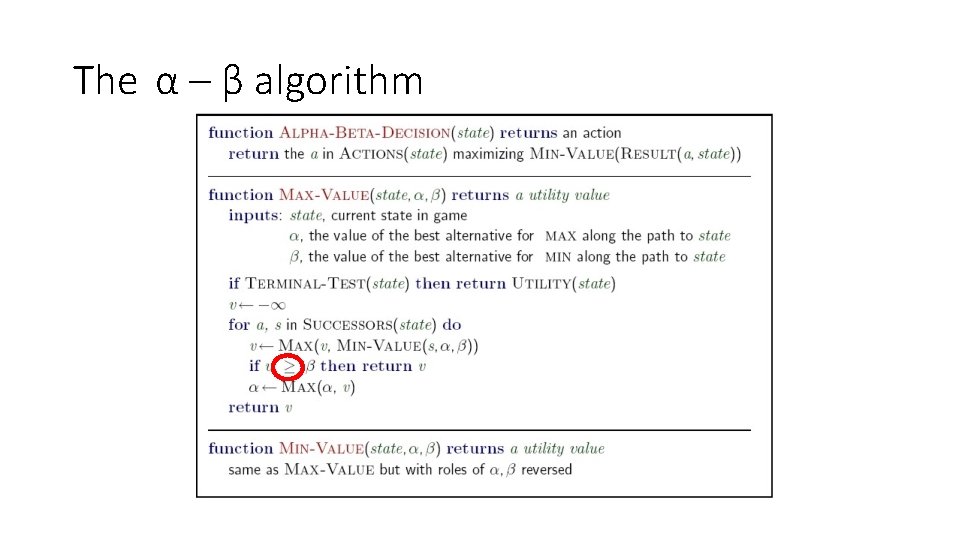
The α – β algorithm

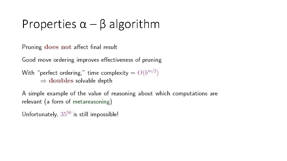
Properties α – β algorithm

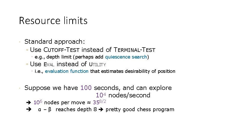
Resource limits · Standard approach: ◦ Use CUTOFF-TEST instead of TERMINAL-TEST · e. g. , depth limit (perhaps add quiescence search) ◦ Use EVAL instead of UTILITY · i. e. , evaluation function that estimates desirability of position · Suppose we have 100 seconds, and can explore 104 nodes/second 106 nodes per move ≈ 358/2 α – β reaches depth 8 pretty good chess program

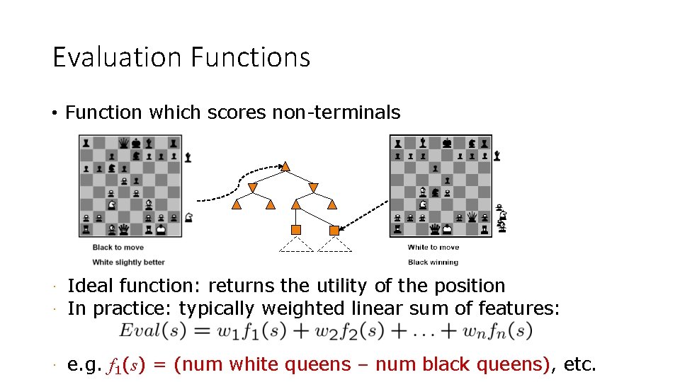
Evaluation Functions • Function which scores non-terminals Ideal function: returns the utility of the position · In practice: typically weighted linear sum of features: · · e. g. f 1(s) = (num white queens – num black queens), etc.

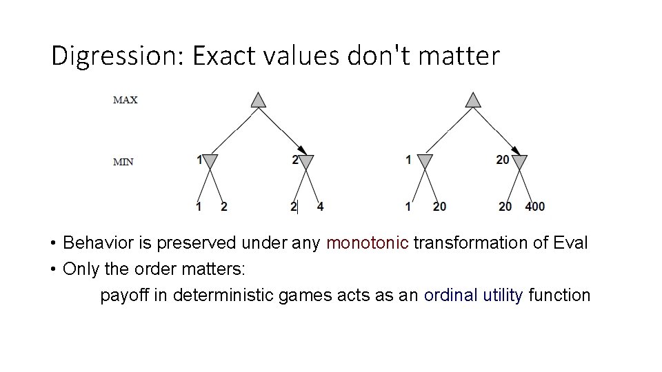
Digression: Exact values don't matter • Behavior is preserved under any monotonic transformation of Eval • Only the order matters: payoff in deterministic games acts as an ordinal utility function

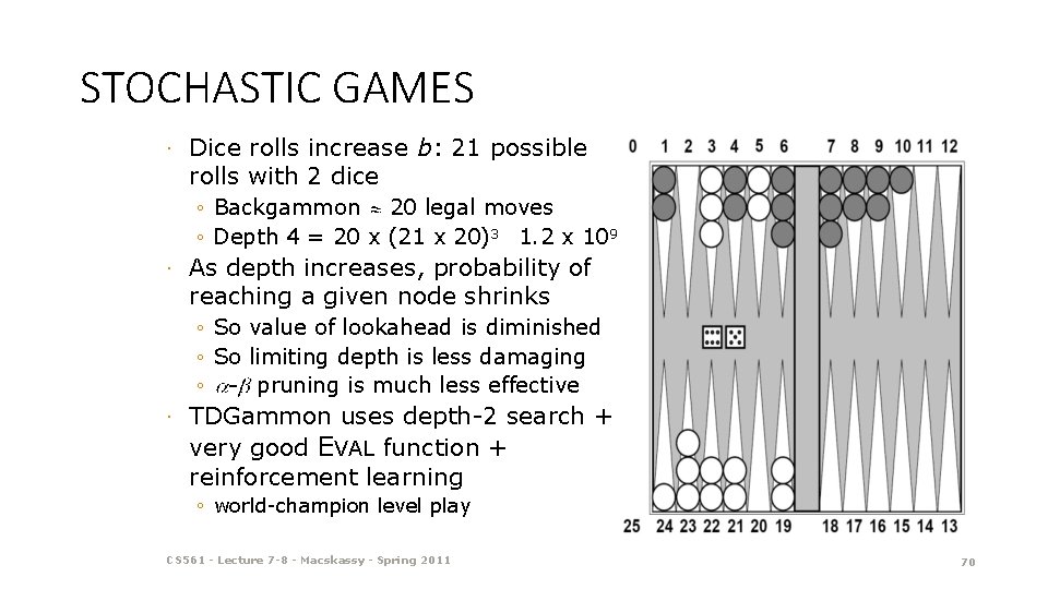
STOCHASTIC GAMES · Dice rolls increase b: 21 possible rolls with 2 dice ◦ Backgammon 20 legal moves ◦ Depth 4 = 20 x (21 x 20)3 1. 2 x 109 · As depth increases, probability of reaching a given node shrinks ◦ So value of lookahead is diminished ◦ So limiting depth is less damaging ◦ - pruning is much less effective · TDGammon uses depth-2 search + very good EVAL function + reinforcement learning ◦ world-champion level play CS 561 - Lecture 7 -8 - Macskassy - Spring 2011 70

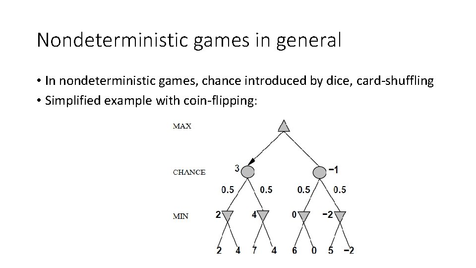
Nondeterministic games in general • In nondeterministic games, chance introduced by dice, card-shuffling • Simplified example with coin-flipping:

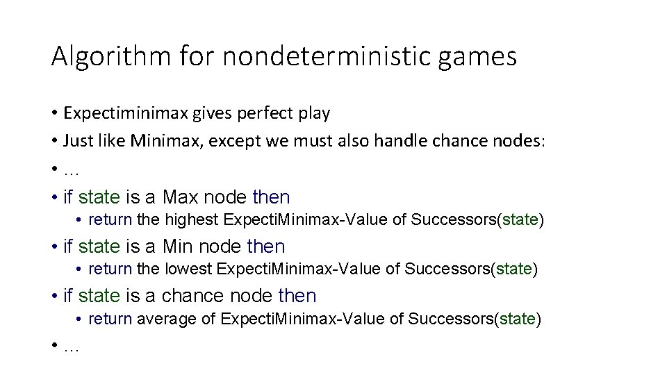
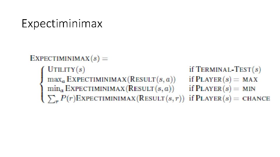
Algorithm for nondeterministic games • Expectiminimax gives perfect play • Just like Minimax, except we must also handle chance nodes: • … • if state is a Max node then • return the highest Expecti. Minimax-Value of Successors(state) • if state is a Min node then • return the lowest Expecti. Minimax-Value of Successors(state) • if state is a chance node then • return average of Expecti. Minimax-Value of Successors(state) • …

Expectiminimax

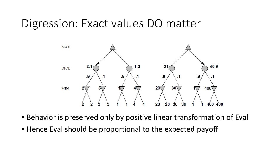
Digression: Exact values DO matter • Behavior is preserved only by positive linear transformation of Eval • Hence Eval should be proportional to the expected payoff

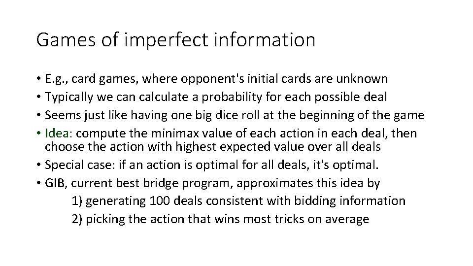
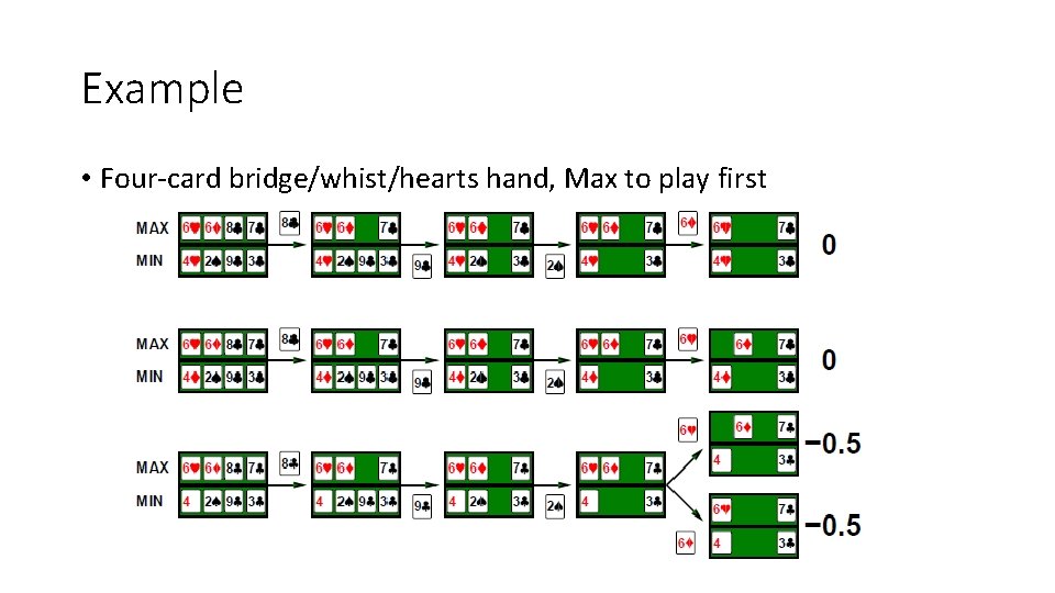
Games of imperfect information • E. g. , card games, where opponent's initial cards are unknown • Typically we can calculate a probability for each possible deal • Seems just like having one big dice roll at the beginning of the game • Idea: compute the minimax value of each action in each deal, then choose the action with highest expected value over all deals • Special case: if an action is optimal for all deals, it's optimal. • GIB, current best bridge program, approximates this idea by 1) generating 100 deals consistent with bidding information 2) picking the action that wins most tricks on average

Example • Four-card bridge/whist/hearts hand, Max to play first

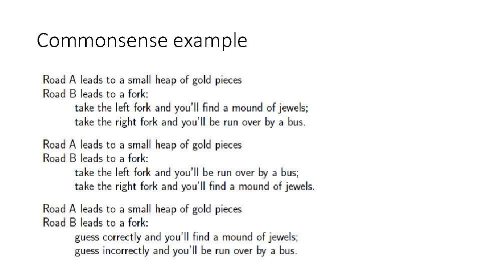
Commonsense example

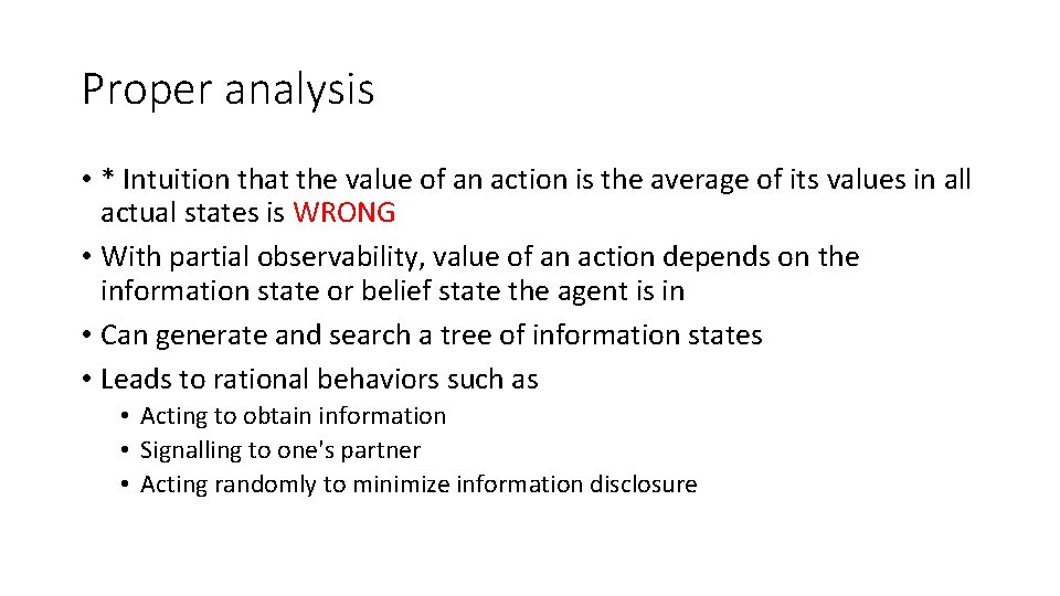
Proper analysis • * Intuition that the value of an action is the average of its values in all actual states is WRONG • With partial observability, value of an action depends on the information state or belief state the agent is in • Can generate and search a tree of information states • Leads to rational behaviors such as • Acting to obtain information • Signalling to one's partner • Acting randomly to minimize information disclosure