Fictitious Play Theory of Learning in Games D

Fictitious Play Theory of Learning in Games D. Fudenberg and D. Levine Speaker: Tzur Sayag 03/06/2003

Do you believe that PM Sharon is serious about the peace process? l l l A voter has to decide if he should support PM Sharon Belief: Sharon will never evacuate settlements • Action: Vote against the new economics revolution. May 24: Sharon announces “occupation is no-good” Belief: Sharon will probably never evacuate settlements • Action: Vote against the new economics revolution Jun 5: Sharon meets Abu-Mazen and declares support for a Palestinian state. l Belief: Seems like Sharon might evacuate the settlements after all • Action: Vote for the new economics revolution.

Roadmap l l Introduction to the common models of learning in games Cournot adjustment Fictitious play and Nash equilibriums • • • Motivation Definitions Results Generalizations of fictitious play – if we have time

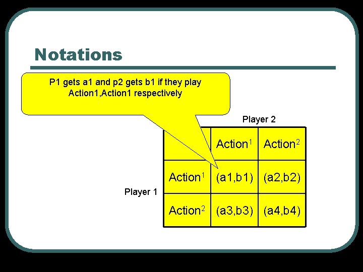
Notations P 1 gets a 1 and p 2 gets b 1 if they play Action 1, Action 1 respectively Player 2 Action 1 Action 2 Action 1 (a 1, b 1) (a 2, b 2) Player 1 Action 2 (a 3, b 3) (a 4, b 4)

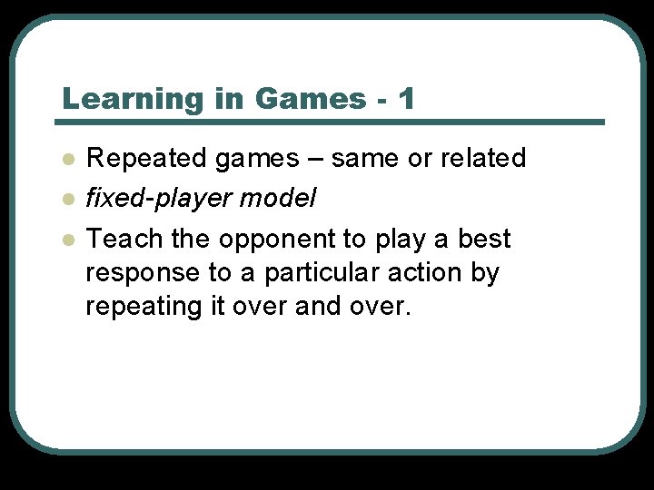
Learning in Games - 1 l l l Repeated games – same or related fixed-player model Teach the opponent to play a best response to a particular action by repeating it over and over.

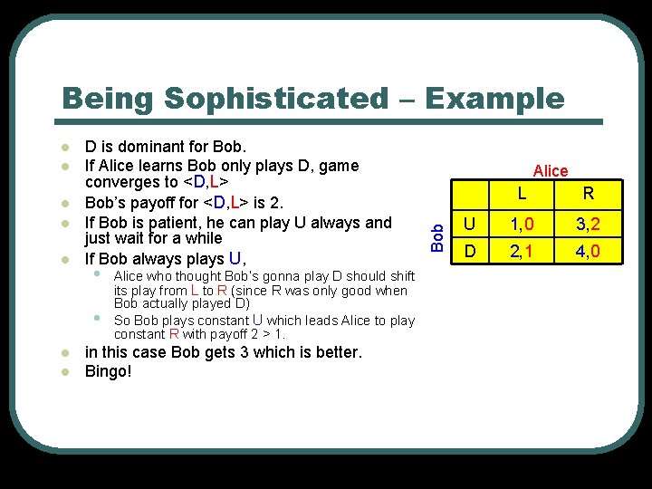
Being Sophisticated – Example l l D is dominant for Bob. If Alice learns Bob only plays D, game converges to <D, L> Bob’s payoff for <D, L> is 2. If Bob is patient, he can play U always and just wait for a while If Bob always plays U, • • l l Alice who thought Bob’s gonna play D should shift its play from L to R (since R was only good when Bob actually played D) So Bob plays constant U which leads Alice to play constant R with payoff 2 > 1. in this case Bob gets 3 which is better. Bingo! Alice Bob l L R U 1, 0 3, 2 D 2, 1 4, 0

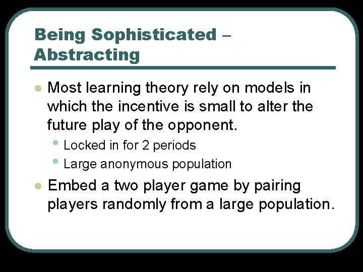
Being Sophisticated – Abstracting l Most learning theory rely on models in which the incentive is small to alter the future play of the opponent. • Locked in for 2 periods • Large anonymous population l Embed a two player game by pairing players randomly from a large population.

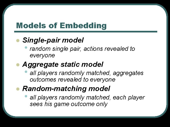
Models of Embedding l Single-pair model • random single pair, actions revealed to everyone l Aggregate static model • all players randomly matched, aggregates outcomes revealed to everyone l Random-matching model • all players randomly matched, each player sees his game outcome only

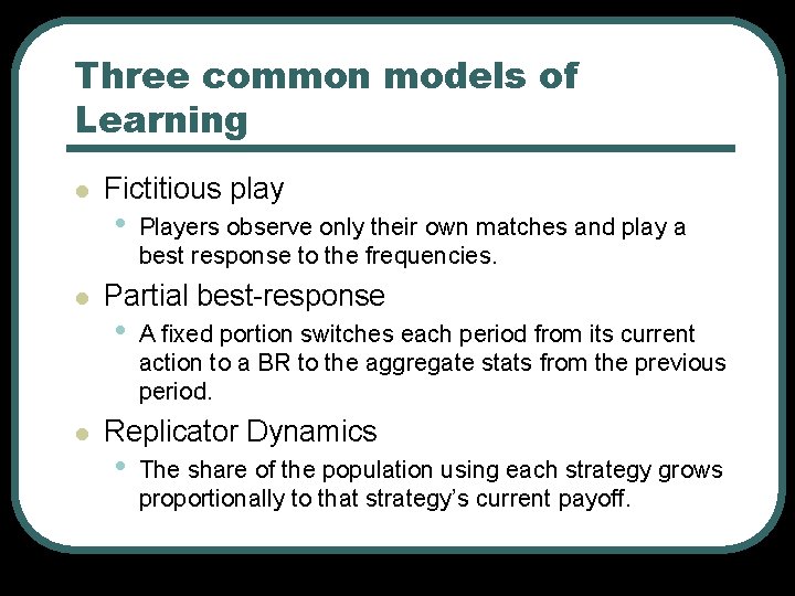
Three common models of Learning l l l Fictitious play • Players observe only their own matches and play a best response to the frequencies. Partial best-response • A fixed portion switches each period from its current action to a BR to the aggregate stats from the previous period. Replicator Dynamics • The share of the population using each strategy grows proportionally to that strategy’s current payoff.

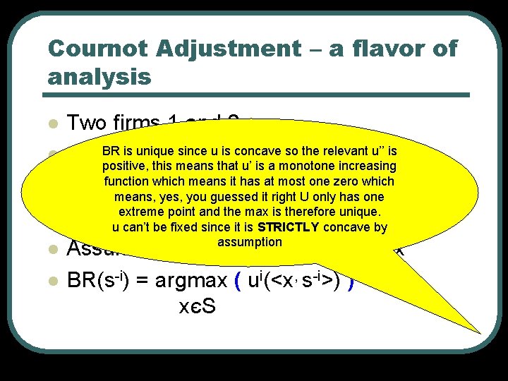
Cournot Adjustment – a flavor of analysis l l l Two firms 1 and 2. iє[0, ∞) BR is unique since u is concave so the relevant u’’ is Strategy: choose a quantity s positive, this means that u’ is a monotone increasing function which means it has at most one zero which i, s-i>єS Strategy profile is <s means, yes, you guessed it right U only has one point and thei, max is therefore unique. i(<s -i>) Utilityuextreme for i is u s can’t be fixed since it is STRICTLY concave by Assume ui(<. , s-iassumption >) is strictly convex BR(s-i) = argmax ( ui(<x, s-i>) ) xєS

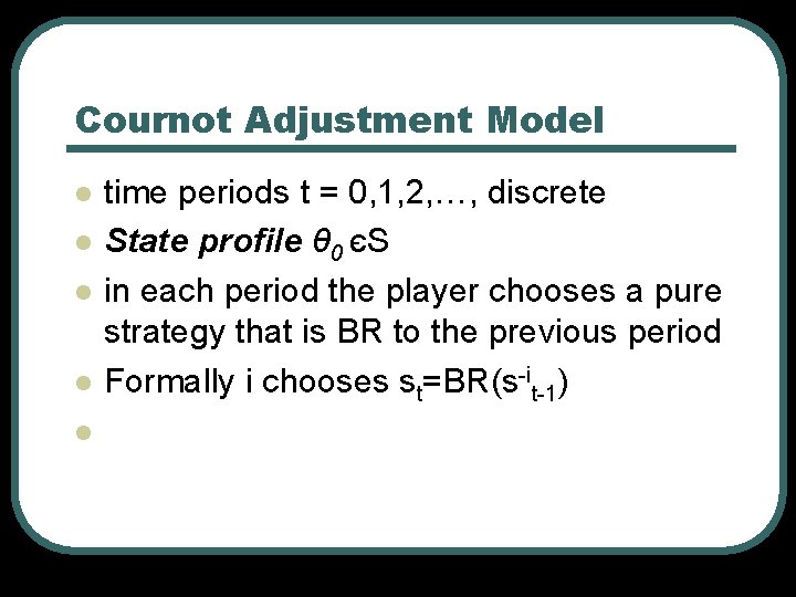
Cournot Adjustment Model l l time periods t = 0, 1, 2, …, discrete State profile θ 0 єS in each period the player chooses a pure strategy that is BR to the previous period Formally i chooses st=BR(s-it-1)

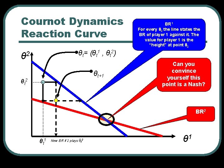
Cournot Dynamics Reaction Curve BR 1 For every θ 2 the line states the BR of player 1 against it. The value for player 1 is the “height” at point θ 2 θt= (θt 1 , θt 2) θ 2 θt+1 θt 2 Can you convince yourself this point is a Nash? BR 2 θt 1 New BR if 2 plays θt 2 θ 1

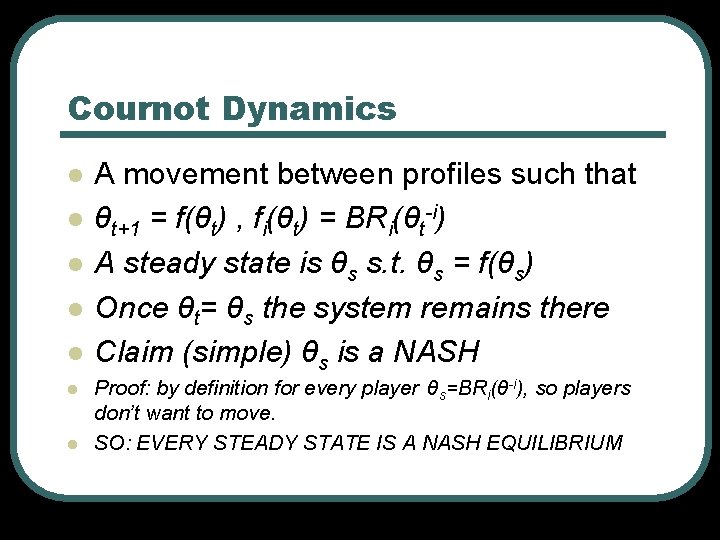
Cournot Dynamics l l l l A movement between profiles such that θt+1 = f(θt) , fi(θt) = BRi(θt-i) A steady state is θs s. t. θs = f(θs) Once θt= θs the system remains there Claim (simple) θs is a NASH Proof: by definition for every player θs=BRi(θ-i), so players don’t want to move. SO: EVERY STEADY STATE IS A NASH EQUILIBRIUM

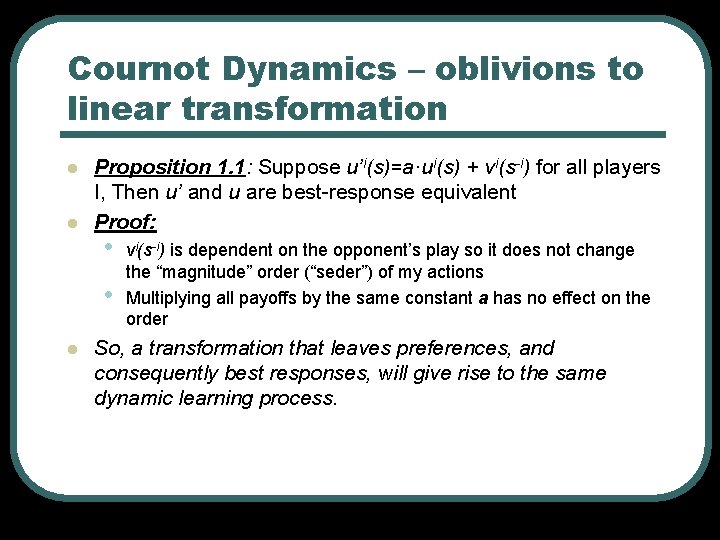
Cournot Dynamics – oblivions to linear transformation l l Proposition 1. 1: Suppose u’i(s)=a·ui(s) + vi(s-i) for all players I, Then u’ and u are best-response equivalent Proof: • • l vi(s-i) is dependent on the opponent’s play so it does not change the “magnitude” order (“seder”) of my actions Multiplying all payoffs by the same constant a has no effect on the order So, a transformation that leaves preferences, and consequently best responses, will give rise to the same dynamic learning process.

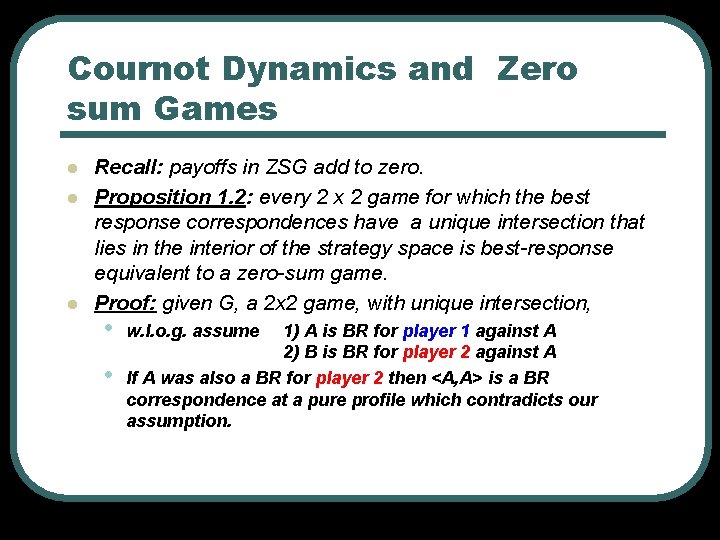
Cournot Dynamics and Zero sum Games l l l Recall: payoffs in ZSG add to zero. Proposition 1. 2: every 2 x 2 game for which the best response correspondences have a unique intersection that lies in the interior of the strategy space is best-response equivalent to a zero-sum game. Proof: given G, a 2 x 2 game, with unique intersection, • • w. l. o. g. assume 1) A is BR for player 1 against A 2) B is BR for player 2 against A If A was also a BR for player 2 then <A, A> is a BR correspondence at a pure profile which contradicts our assumption.

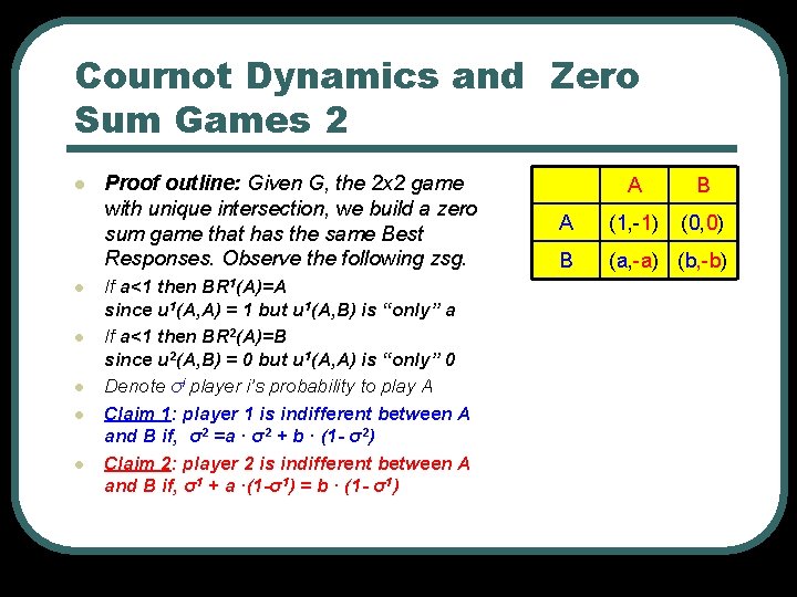
Cournot Dynamics and Zero Sum Games 2 l l l Proof outline: Given G, the 2 x 2 game with unique intersection, we build a zero sum game that has the same Best Responses. Observe the following zsg. If a<1 then BR 1(A)=A since u 1(A, A) = 1 but u 1(A, B) is “only” a If a<1 then BR 2(A)=B since u 2(A, B) = 0 but u 1(A, A) is “only” 0 Denote σi player i’s probability to play A Claim 1: player 1 is indifferent between A and B if, σ2 =a · σ2 + b · (1 - σ2) Claim 2: player 2 is indifferent between A and B if, σ1 + a ·(1 -σ1) = b · (1 - σ1) A B A (1, -1) (0, 0) B (a, -a) (b, -b)

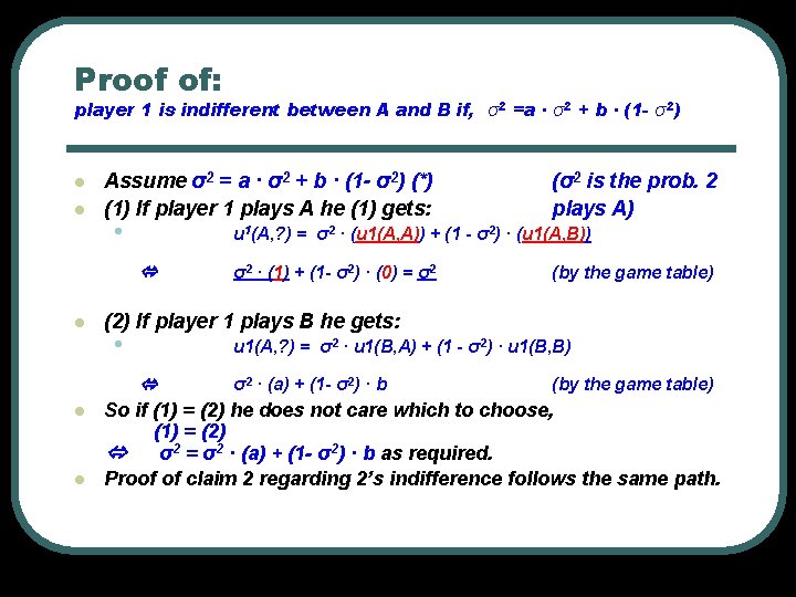
Proof of: player 1 is indifferent between A and B if, σ2 =a · σ2 + b · (1 - σ2) l l Assume σ2 = a · σ2 + b · (1 - σ2) (*) (1) If player 1 plays A he (1) gets: • u 1(A, ? ) = σ2 · (u 1(A, A)) + (1 - σ2) · (u 1(A, B)) l l σ2 · (1) + (1 - σ2) · (0) = σ2 (by the game table) (2) If player 1 plays B he gets: • u 1(A, ? ) = σ2 · u 1(B, A) + (1 - σ2) · u 1(B, B) l (σ2 is the prob. 2 plays A) σ2 · (a) + (1 - σ2) · b (by the game table) So if (1) = (2) he does not care which to choose, (1) = (2) σ2 = σ2 · (a) + (1 - σ2) · b as required. Proof of claim 2 regarding 2’s indifference follows the same path.

Mental note: σ = Pr[player i playing A] Proof cont: Building the ZSG Game i l l 1 is indifferent between A and B if σ2 =a · σ2 + b · (1 - σ2) 2 is indifferent between A and B if σ1 + a ·(1 -σ1) = b · (1 - σ1) Fixing an intersection point σ1, σ2 We can solve for the unknown payoffs a, b: a= (σ2 – σ1) / (1+ σ2 · σ1) Notice that (σ2 – σ1) < 1 (σi > 0 otherwise i never plays A…) (σ2 – σ1) < 1 implies a<1 (since (1+ σ2 · σ1)>1) Q. E. D. We already showed that when a< 1 it means that we get the same best responses we had in the original game G: A for player 1 against A, B for player 2 against A l To sum up: it should have been obvious that (σ1, σ2 ) is a Nash, the point was to find a 2 x 2 ZSG which has the same best responses as the original game

Strategic-Form Games l l l Finite actions One shot simultaneous-move games {Players, strategy space, payoff functions} is the strategic form of a game

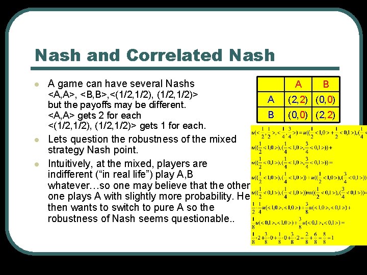
Nash and Correlated Nash l A game can have several Nashs <A, A>, <B, B>, <(1/2, 1/2), (1/2, 1/2)> but the payoffs may be different. <A, A> gets 2 for each <(1/2, 1/2), (1/2, 1/2)> gets 1 for each. l l Lets question the robustness of the mixed strategy Nash point. Intuitively, at the mixed, players are indifferent (“in real life”) play A, B whatever…so one may believe that the other one plays A with slightly more probability. He then wants to switch to pure A so the robustness of Nash seems questionable. . A B A (2, 2) (0, 0) B (0, 0) (2, 2)

Nash and Correlated Nash l l l A Nash is strict if for each player i, si is the unique best response to s-i Only pure strategies can be strict since if a mixed is BR than so is every pure strategy in the mixed strategy’s support otherwise there is no point of including it. Recall: Support for a mixed strategy are the pure strategies that participate with positive probability.

Some Questions in Theory of Games l l l When and why should we expect play to correspond to a Nash equilibrium If there are several Nash equilibria, when one should we expect to occur? In the previous example, in the absence of coordination, we are faced with the possibility that player 1 expects NE 1=<A, A> so he plays A, the opponent might expect NE 2=<B, B> and he plays B, with the results of the nonequilibrium outcome profile <A, B>

The Idea of Learning based explanation of equilibrium l l Intuitively, the history of observations can provide a way for the players to coordinate their expectations on one of the two pure-strategy equilibrium. Typically, Learning models predict that this coordination will eventually occur, with the determination of which of the two eq. arise left to initial conditions or to random chance.

The Idea of Learning based explanation of equilibrium l l For the history to serve this coordination role, the sequence of actions played must eventually become constant or at least readily predictable by the players, of course, there is no presumption that this is always the case. Perhaps, rather than going to a Nash, players wander around the space aimlessly, or perhaps play lies in some set of alternatives larger than the set of Nashs?

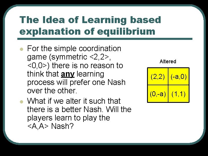
The Idea of Learning based explanation of equilibrium l l For the simple coordination game (symmetric <2, 2>, <0, 0>) there is no reason to think that any learning process will prefer one Nash over the other. What if we alter it such that there is a better Nash. Will the players learn to play the <A, A> Nash? Altered (2, 2) (-a, 0) (0, -a) (1, 1)

Correlated Nash (Aumann 74) l l l Suppose the players have access to randomized devices that are privately viewed. If a player chooses a strategy according to his own randomized device, the result is a probability distribution over strategy profiles, denoted μєΔ(S). Unlike a profile of mixed strategies which is by definition uncorrelated, such a distribution may be correlated.

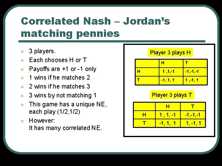
Correlated Nash – Jordan’s matching pennies l l l l 3 players. Each chooses H or T Payoffs are +1 or -1 only 1 wins if he matches 2 2 wins if he matches 3 3 wins by not matching 1 This game has a unique NE, each play (1/2, 1/2) However: It has many correlated NE. Player 3 plays H H T H 1 , 1, -1 -1, -1 T -1, 1, 1 1 , -1, 1 Player 3 plays T H 1 , 1, -1 -1, -1 T -1, 1, 1 1, -1, 1

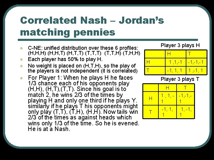
Correlated Nash – Jordan’s matching pennies l l C-NE: unified distribution over these 6 profiles: (H, H, H) (H, H, T) (H, T, T) (T, T, H) (T, H, H) Each player has 50% to play H. No weight is placed on (H, T, H), so the play of the players is not independent (it is correlated) For Player 1: When he plays H he faces 1/3 chance each of his opponents play (H, H), (H, T), (T, T). Since his goal is to match 2, he wins 2/3 of the times by playing H and only one third if he plays Y. similarly if he plays T his opponents might only play (T, T), (T, H), (H, H). Now tails win 2/3 of the times as against heads which wins only 1/3 of the time. So he is evened. He is at a Nash. Player 3 plays H H T H 1 , 1, -1 -1, -1 T -1, 1, 1 1 , -1, 1 Player 3 plays T H 1 , 1, 1 -1, 1 T -1, 1, 1 1, -1, 1

Why is Correlated Nash of Significance? l l Hint – Cycles create correlation between profile strategies. Informally a cycle is a finite sequence of profiles of length k such that s 0=sk. Cournot play can exhibit cycles – example follows. So cycles => correlation => correlated Nash

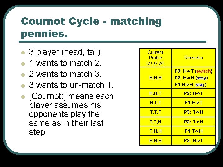
Cournot Cycle - matching pennies. l l l 3 player (head, tail) 1 wants to match 2. 2 wants to match 3. 3 wants to un-match 1. [Cournot: ] means each player assumes his opponents play the same as in their last step Current Profile (s 1, s 2, s 3) Remarks H, H, H P 3: H->T (switch) P 2: H->H (stay) P 1: H->H (stay) H, H, T P 2: H->T H, T, T P 1: H->T T, T, T P 3: T->H T, T, H P 2: T->H T, H, H P 1: T->H H, H, H P 3: H->T

Roadmap l Introduction to the common models of learning Cournot adjustment Fictitious play and Nash equilibriums l Generalizations of fictitious play l l • Motivation • Definitions • Results

Fictitious play - Introduction l l Motivation… Repeated game, stationary assumption…. Each player forms a belief of his opponents “strategy” by looking at what happened Player plays Best Response according to his/her belief

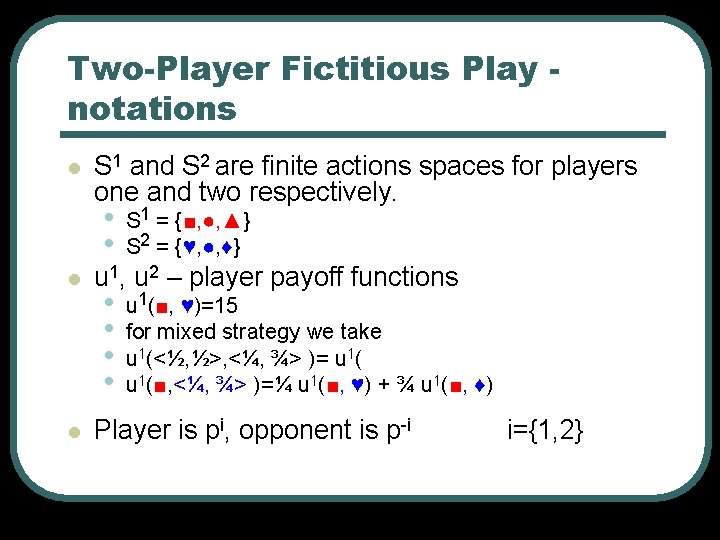
Two-Player Fictitious Play notations l S 1 and S 2 are finite actions spaces for players one and two respectively. • • S 1 = {■, ●, ▲} S 2 = {♥, ●, ♦} • • u 1(■, ♥)=15 for mixed strategy we take u 1(<½, ½>, <¼, ¾> )= u 1(■, <¼, ¾> )=¼ u 1(■, ♥) + ¾ u 1(■, ♦) l u 1, u 2 – player payoff functions l Player is pi, opponent is p-i i={1, 2}

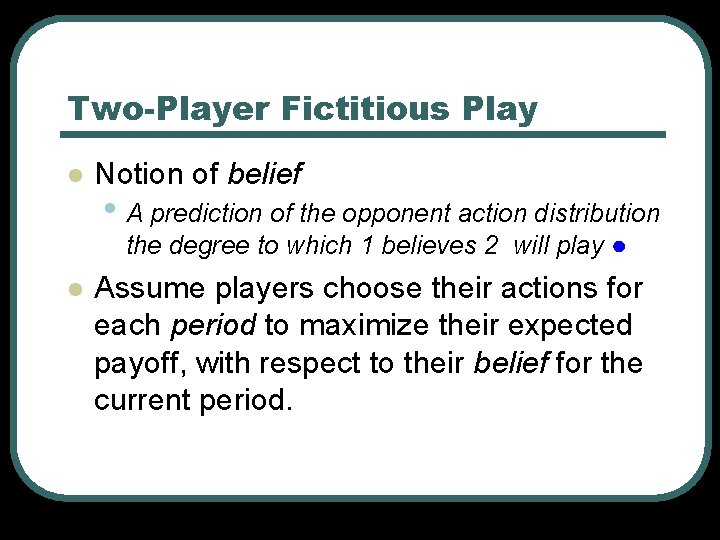
Two-Player Fictitious Play l Notion of belief • A prediction of the opponent action distribution the degree to which 1 believes 2 will play ● l Assume players choose their actions for each period to maximize their expected payoff, with respect to their belief for the current period.

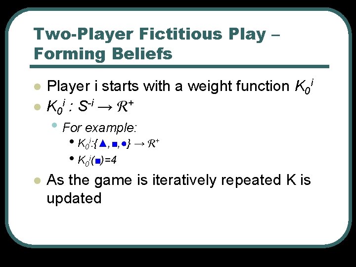
Two-Player Fictitious Play – Forming Beliefs l l Player i starts with a weight function K 0 i : S-i → + • For example: • K 0 i: {▲, ■, ●} → + • K 0 i(■)=4 l As the game is iteratively repeated K is updated

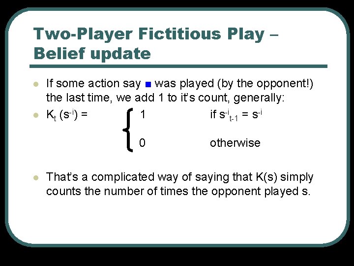
Two-Player Fictitious Play – Belief update l l If some action say ■ was played (by the opponent!) the last time, we add 1 to it’s count, generally: Kt (s-i) = 1 if s-it-1 = s-i 0 l otherwise That’s a complicated way of saying that K(s) simply counts the number of times the opponent played s.

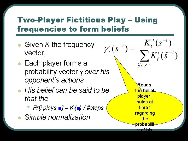
Two-Player Fictitious Play – Using frequencies to form beliefs l l l Given K the frequency vector, Each player forms a probability vector over his opponent’s actions His belief can be said to be that the • l Pr[i plays ■] = Kt(■) / #steps Simple normalization Reads: the belief player i holds at time t regarding the probabilit y of his opponent

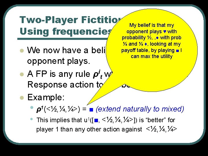
Two-Player Fictitious. My. Play – belief is that my Using frequencies 2 opponent plays ♥ with l l l probability ½, , ● with prob ¼ and ¼ ♦, looking at my payoff table, by playing ■ I can max the utility We now have a belief of how the opponent plays. A FP is any rule ρit which assigns a Best Response action to the belief it Example: • ρ1(<½, ¼, ¼>) = ■ (extend naturally to mixed) • This implies that u 1([■, <½, ¼, ¼>]) is “better” for player 1 than any other action against <½, ¼, ¼>

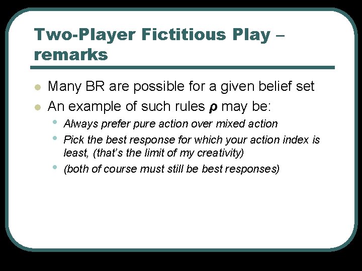
Two-Player Fictitious Play – remarks l l Many BR are possible for a given belief set An example of such rules ρ may be: • • • Always prefer pure action over mixed action Pick the best response for which your action index is least, (that’s the limit of my creativity) (both of course must still be best responses)

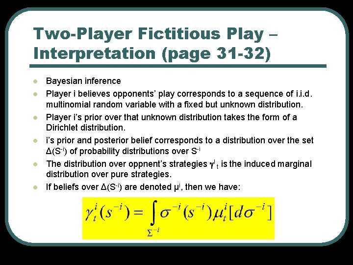
Two-Player Fictitious Play – Interpretation (page 31 -32) l l l Bayesian inference Player i believes opponents’ play corresponds to a sequence of i. i. d. multinomial random variable with a fixed but unknown distribution. Player i’s prior over that unknown distribution takes the form of a Dirichlet distribution. i’s prior and posterior belief corresponds to a distribution over the set Δ(S-i) of probability distributions over S-i The distribution over oppnent’s strategies I t is the induced marginal distribution over pure strategies. If beliefs over Δ(S-i) are denoted μi, then we have:

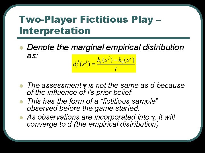
Two-Player Fictitious Play – Interpretation l Denote the marginal empirical distribution as: l The assessment is not the same as d because of the influence of i’s prior belief This has the form of a “fictitious sample” observed before the game started. As observations are incorporated into , it will converge to d (the empirical distribution) l l

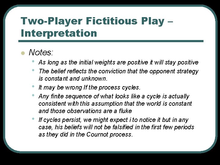
Two-Player Fictitious Play – Interpretation l Notes: • • • As long as the initial weights are positive it will stay positive The belief reflects the conviction that the opponent strategy is constant and unknown. It may be wrong If the process cycles. Any finite sequence of what looks like a cycle is actually consistent with this assumption that the world is constant and those observations are a fluke If cycles persist, we might expect i to notice it but in any case, his beliefs will not be falsified in the first few periods as they did in the Cournot process.

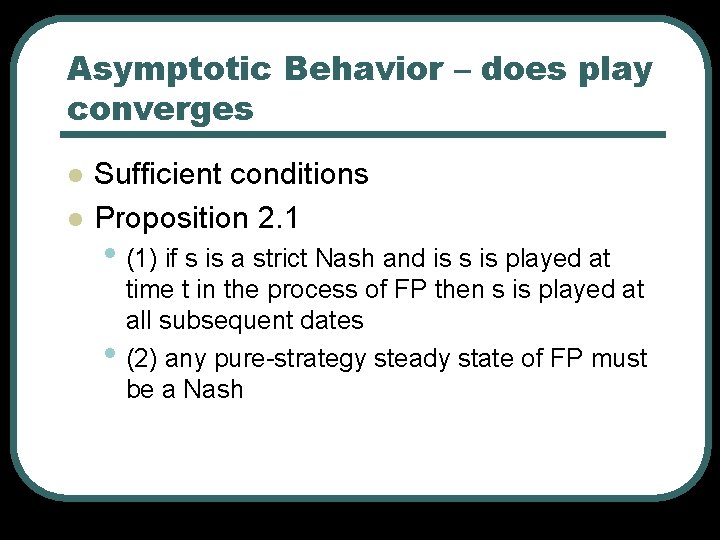
Asymptotic Behavior – does play converges l l Sufficient conditions Proposition 2. 1 • (1) if s is a strict Nash and is s is played at • time t in the process of FP then s is played at all subsequent dates (2) any pure-strategy steady state of FP must be a Nash

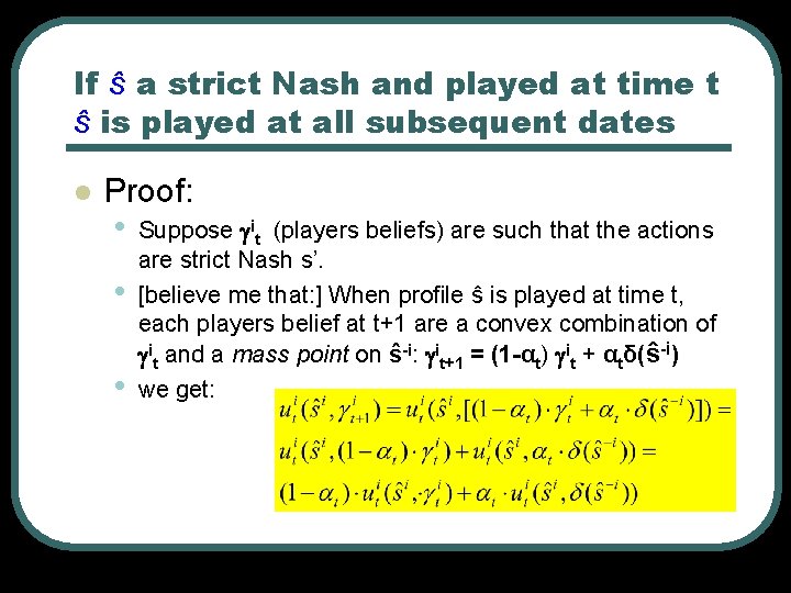
If ŝ a strict Nash and played at time t ŝ is played at all subsequent dates l Proof: • • • Suppose it (players beliefs) are such that the actions are strict Nash s’. [believe me that: ] When profile ŝ is played at time t, each players belief at t+1 are a convex combination of it and a mass point on ŝ-i: it+1 = (1 -αt) it + αtδ(ŝ-i) we get:

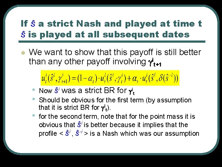
If ŝ a strict Nash and played at time t ŝ is played at all subsequent dates l We want to show that this payoff is still better than any other payoff involving it+1 • • • Now ŝi was a strict BR for it Should be obvious for the first term (by assumption that it is strict BR for it). for the second term, note that for the point mass it is obvious that ŝi is better because it implies that the profile < ŝi , ŝ-i > is a Nash which was our assumption

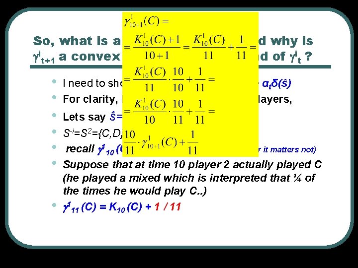
So, what is a point mass on ŝ-i and why is it+1 a convex combination of it and of it ? • • I need to show you that: it+1 = (1 -αt) it + αtδ(ŝ) For clarity, lets say t=10, there are 2 players, Lets say ŝ={( ½, ½ ), ( ¼ , ¾ )} S-i=S 2={C, D} and look at 110+1(C) recall 110 (C)=K 10 (C) /10 (ignore prior it matters not) Suppose that at time 10 player 2 actually played C (he played a mixed which is interpreted that ¼ of the times he would play C. . ) 111 (C) = K 10 (C) + 1 / 11

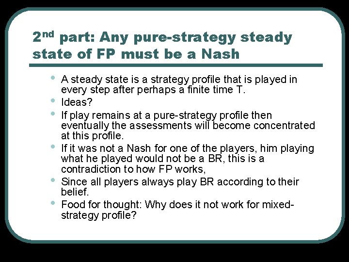
2 nd part: Any pure-strategy steady state of FP must be a Nash • • • A steady state is a strategy profile that is played in every step after perhaps a finite time T. Ideas? If play remains at a pure-strategy profile then eventually the assessments will become concentrated at this profile. If it was not a Nash for one of the players, him playing what he played would not be a BR, this is a contradiction to how FP works, Since all players always play BR according to their belief. Food for thought: Why does it not work for mixedstrategy profile?

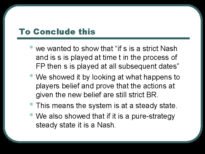
To Conclude this • we wanted to show that “if s is a strict Nash • • • and is s is played at time t in the process of FP then s is played at all subsequent dates” We showed it by looking at what happens to players belief and prove that the actions at given the new belief are still strict BR. This means the system is at a steady state. We also showed that if it is a pure-strategy steady state it is a Nash.

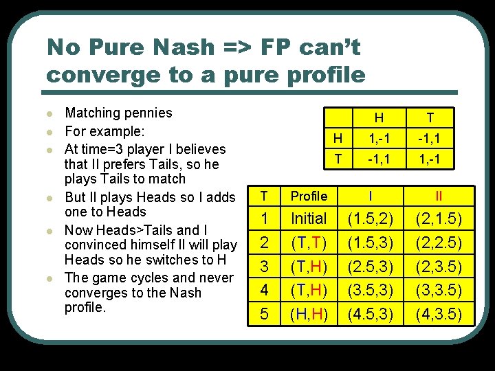
No Pure Nash => FP can’t converge to a pure profile l l l Matching pennies For example: At time=3 player I believes that II prefers Tails, so he plays Tails to match But II plays Heads so I adds one to Heads Now Heads>Tails and I convinced himself II will play Heads so he switches to H The game cycles and never converges to the Nash profile. H T H 1, -1 -1, 1 T -1, 1 1, -1 T Profile I II 1 Initial (1. 5, 2) (2, 1. 5) 2 (T, T) (1. 5, 3) (2, 2. 5) 3 (T, H) (2. 5, 3) (2, 3. 5) 4 (T, H) (3. 5, 3) (3, 3. 5) 5 (H, H) (4. 5, 3) (4, 3. 5)

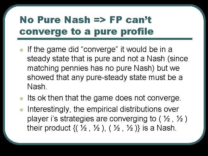
No Pure Nash => FP can’t converge to a pure profile l l l If the game did “converge” it would be in a steady state that is pure and not a Nash (since matching pennies has no pure Nash) but we showed that any pure-steady state must be a Nash. Its ok then that the game does not converge. Interestingly, the empirical distributions over player i’s strategies are converging to ( ½ , ½ ) their product {( ½ , ½ ), ( ½ , ½ )} is a Nash.

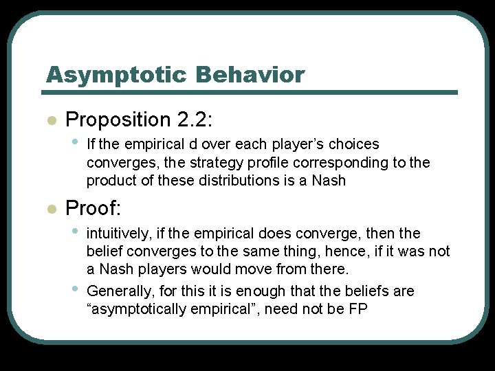
Asymptotic Behavior l l Proposition 2. 2: • If the empirical d over each player’s choices converges, the strategy profile corresponding to the product of these distributions is a Nash Proof: • • intuitively, if the empirical does converge, then the belief converges to the same thing, hence, if it was not a Nash players would move from there. Generally, for this it is enough that the beliefs are “asymptotically empirical”, need not be FP

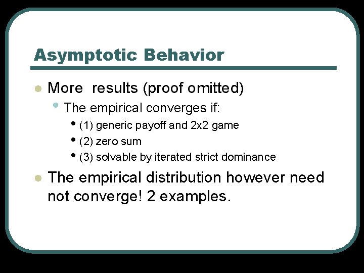
Asymptotic Behavior l More results (proof omitted) • The empirical converges if: • (1) generic payoff and 2 x 2 game • (2) zero sum • (3) solvable by iterated strict dominance l The empirical distribution however need not converge! 2 examples.

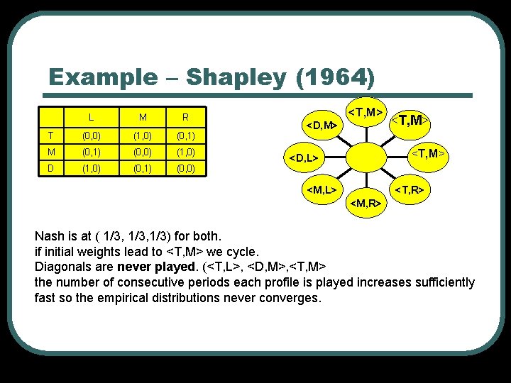
Example – Shapley (1964) L M R T (0, 0) (1, 0) (0, 1) M (0, 1) (0, 0) (1, 0) D (1, 0) (0, 1) (0, 0) <T, M> <D, M> <T, M> <D, L> <M, L> <T, R> <M, R> Nash is at ( 1/3, 1/3) for both. if initial weights lead to <T, M> we cycle. Diagonals are never played. (<T, L>, <D, M>, <T, M> the number of consecutive periods each profile is played increases sufficiently fast so the empirical distributions never converges.

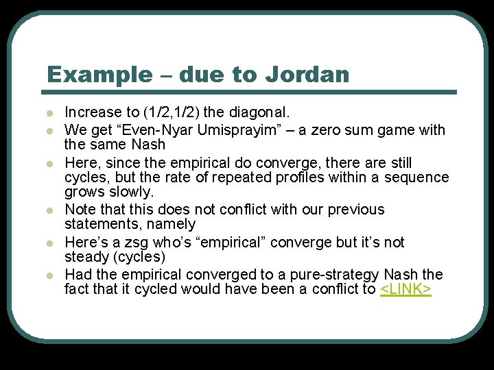
Example – due to Jordan l l l Increase to (1/2, 1/2) the diagonal. We get “Even-Nyar Umisprayim” – a zero sum game with the same Nash Here, since the empirical do converge, there are still cycles, but the rate of repeated profiles within a sequence grows slowly. Note that this does not conflict with our previous statements, namely Here’s a zsg who’s “empirical” converge but it’s not steady (cycles) Had the empirical converged to a pure-strategy Nash the fact that it cycled would have been a conflict to <LINK>

Payoffs in Fictitious Play l l The question we deal with here is if FP “learns” the distributions then it should, asymptotically yield the same utility that would be achieved when the frequency distribution is known in advance. Here we will suppose more than 2 players, their assessment track the joint distribution of opponent strategies.

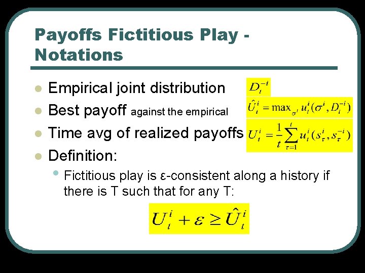
Payoffs Fictitious Play Notations l l Empirical joint distribution Best payoff against the empirical Time avg of realized payoffs Definition: • Fictitious play is ε-consistent along a history if there is T such that for any T:

Payoffs Fictitious Play Notations l l Empirical joint distribution Best payoff against the empirical Time avg of realized payoffs Definition: • Fictitious play is ε-consistent along a history if there is T such that for any T:

Consistency l l We don’t look at how good the player does globally but how good he does with comparison to his expectations which are built upon his beliefs. If the FP is not consistent it would be much less interesting model, it would be as if someone simply plays a different game. So, we want consistency.

Consistency l If A game is consistent it can be useful, if after some period of time, a player sees that his expectations are not fulfilled (by comparing the expected payoff with the actual payoff), he can deduce that something is wrong in his model of the world.

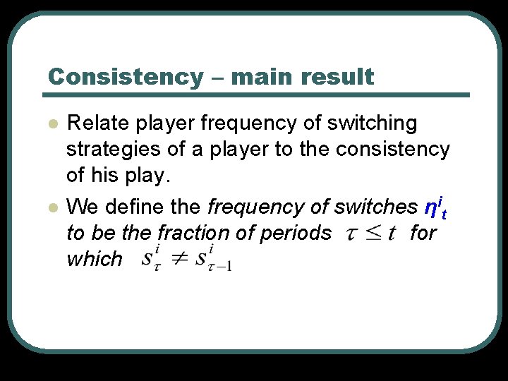
Consistency – main result l l Relate player frequency of switching strategies of a player to the consistency of his play. We define the frequency of switches ηit to be the fraction of periods for which

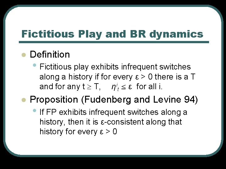
Fictitious Play and BR dynamics l Definition • Fictitious play exhibits infrequent switches along a history if for every ε > 0 there is a T and for any t T, ηit ε for all i. l Proposition (Fudenberg and Levine 94) • If FP exhibits infrequent switches along a history, then it is ε-consistent along that history for every ε > 0

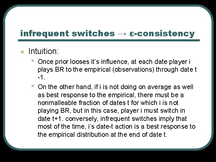
infrequent switches → ε-consistency l Intuition: • • Once prior looses it’s influence, at each date player i plays BR to the empirical (observations) through date t -1. On the other hand, if i is not doing on average as well as best response to the empirical, there must be a nonmalleable fraction of dates t for which i is not playing BR, but in this case, player i must switch in date t+1. conversely, infrequent switches imply that most of the time, i’s date-t action is a best response to the empirical distribution at the end of date t.

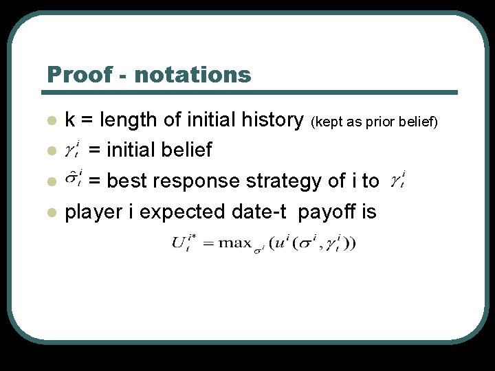
Proof - notations l l k = length of initial history (kept as prior belief) = initial belief = best response strategy of i to player i expected date-t payoff is

Proof - summary l l l We showed that if there are not many switches along the players history, his play is consistent. It means that the actual payoffs do not flounder below the expectation! Again, one can use this to see if something is wrong with his model of the env.

Roadmap l Crash introduction to the common models of learning Cournot adjustment Fictitious play and Nash equilibriums l Generalizations of fictitious play l l • Motivation • Definitions • Results

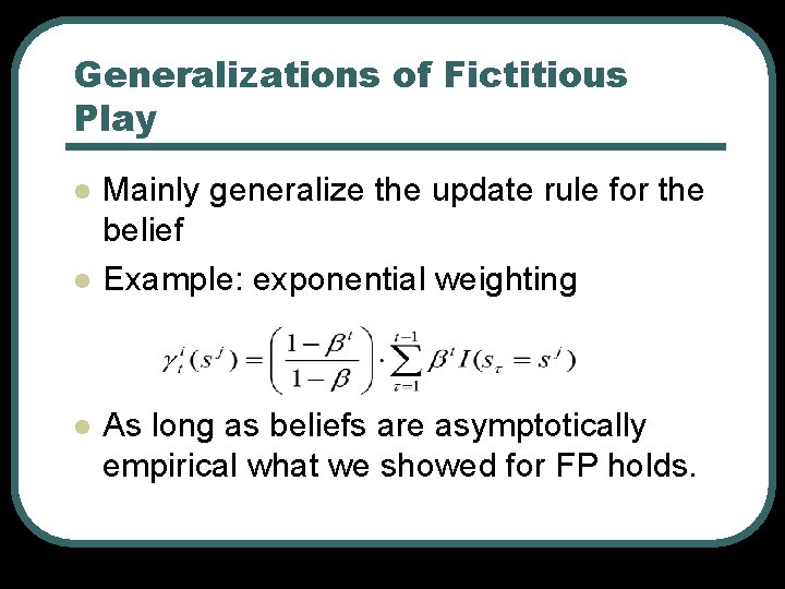
Generalizations of Fictitious Play l l l Mainly generalize the update rule for the belief Example: exponential weighting As long as beliefs are asymptotically empirical what we showed for FP holds.

Summary l l Dynamics of Games and a flavor of analysis Although different from Nash analysis, Nash is still an important point, we showed that it is still a point FP can converge to FP is a consistent play Have a nice summer vacation & thanx for listening.