Advanced Computer Vision Chapter 3 Image Processing Presented

Advanced Computer Vision Chapter 3 Image Processing Presented by: 傅楸善 & 黃季軒 0935090120 tazdingohuang@gmail. com 1

Image Processing • • 3. 1 Point Operators 3. 2 Linear Filtering 3. 3 More Neighborhood Operators 3. 4 Fourier Transforms 3. 5 Pyramids and Wavelets 3. 6 Geometric Transformations 3. 7 Global Optimization 2

3

4

3. 1. 1 Pixel Transforms (1/5) • • x is in the D-dimensional domain of the functions (usually D = 2 for images) and the functions f and g operate over some range, which can either be scalar or vector-valued, e. g. , for color images or 2 D motion. • For discrete images, the domain consists of a finite number of pixel locations, x = (i, j), and we can write 5

3. 1. 1 Pixel Transforms (2/5) • before after 6

3. 1. 1 Pixel Transforms (3/5) • Multiplication and addition with a constant • The parameters a > 0 and b are often called the gain and bias parameters. • The bias and gain parameters can also be spatially varying. 7

3. 1. 1 Pixel Transforms (4/5) • Multiplicative gain is a linear operation • Non-linear transform: gamma correction 8

3. 1. 1 Pixel Transforms (5/5) • Dyadic (two-input) operator is the linear blend operator 9

3. 1. 2 Color Transforms • In fact, adding the same value to each color channel not only increases the apparent intensity of each pixel, it can also affect the pixel’s hue and saturation. 10

3. 1. 3 Compositing and Matting (1/4) • In many photo editing and visual effects applications, it is often desirable to cut a foreground object out of one scene and put it on top of a different background. • The process of extracting the object from the original image is often called matting, while the process of inserting it into another image (without visible artifacts) is called compositing. 11

3. 1. 3 Compositing and Matting (2/4) • Alpha-matted color image – In addition to the three color RGB channels, an alphamatted image contains a fourth alpha channel α (or A) that describes the relative amount of opacity or fractional coverage at each pixel. – Pixels within the object are fully opaque (α= 1), while pixels fully outside the object are transparent (α= 0). 12

3. 1. 3 Compositing and Matting (3/4) 13

3. 1. 3 Compositing and Matting (4/4) 14

3. 1. 4 Histogram Equalization • To find an intensity mapping function f(I) such that the resulting histogram is flat – h(I): original histogram – c(I): cumulative distribution – N: the number of pixels in the image • A linear blend between the cumulative distribution function and the identity transform 15

16

Locally Adaptive Histogram Equalization (1/4) • Subdivide the image into M×M pixel blocks and perform separate histogram equalization in each sub-block. • But the resulting image exhibits a lot of blocking artifacts, i. e. , intensity discontinuities at block boundaries. 17

18

Locally Adaptive Histogram Equalization (2/4) • One way to eliminate blocking artifacts is to use a moving window, i. e. , to recompute the histogram for every M×M block centered at each pixel. • A more efficient approach is to compute nonoverlapped block-based equalization functions as before, but to then smoothly interpolate the transfer functions as we move between blocks. This technique is known as adaptive histogram equalization (AHE). 19

Locally Adaptive Histogram Equalization (3/4) • Adaptive Histogram Equalization (AHE) • The weighting function for a given pixel (i, j) can be computed as a function of its horizontal and vertical position (s, t) within a block. • To blend the four lookup {f 00, …, f 11}, a bilinear blending function 20

21

1 -t f 01 f 02 f 10 f 11 f 12 f 20 f 21 f 22 f 00 t s 1 -s 22

f 00 t 1 -t f 01 s 1 -s f 10 f 11 23

Image Processing • • 3. 1 Point Operators 3. 2 Linear Filtering 3. 3 More Neighborhood Operators 3. 4 Fourier Transforms 3. 5 Pyramids and Wavelets 3. 6 Geometric Transformations 3. 7 Global Optimization 24

25

3. 2 Linear Filtering • An output pixel’s value is determined as a weighted sum of input pixel values. • • 26

27

28

29

• A one-dimensional convolution can be represented in matrix-vector form. 30

Padding (Border Effects) • zero: set all pixels outside the source image to 0. • constant (border color): set all pixels outside the source image to a specified border value. • clamp (replicate or clamp to edge): repeat edge pixels indefinitely • mirror: reflect pixels across the image edge • (cyclic) wrap (repeat or tile): loop “around” the image in a toroidal configuration 31

32

3. 2. 1 Separable Filtering (1/2) • The process of performing a convolution requires K 2 operations per pixel, where K is the size (width or height) of the convolution kernel. • This operation can be significantly sped up by first performing a one-dimensional horizontal convolution followed by a one-dimensional vertical convolution (which requires a total of 2 K operations per pixel). 33

3. 2. 1 Separable Filtering (2/2) • It is easy to show that the two-dimensional kernel K corresponding to successive convolution with a horizontal kernel h and a vertical kernel v is the outer product of the two kernels, 34

3. 2. 2 Examples of Linear Filtering • The simplest filter to implement is the moving average or box filter, which simply averages the pixel values in a K×K window. 35

36

3. 2. 3 Band-Pass and Steerable Filters (1/3) • The (undirected) second derivative of a twodimensional image is known as the Laplacian operator. • Blurring an image with a Gaussian and then taking its Laplacian is equivalent to convolving directly with the Laplacian of Gaussian (Lo. G) filter. http: //fourier. eng. hmc. edu/e 161/lectures/gradient/node 8. html 37

3. 2. 3 Band-Pass and Steerable Filters (2/3) • The Sobel operator is a simple approximation to a directional or oriented filter, which can be obtained by smoothing with a Gaussian (or some other filter) and then taking a directional derivative , which is obtained by taking the dot product between the gradient field and a unit direction 38

3. 2. 3 Band-Pass and Steerable Filters (3/3) • The smoothed directional derivative filter, • is an example of a steerable filter, since the value of an image convolved with can be computed by first convolving with the pair of filters (Gx, Gy) and then steering the filter by multiplying this gradient field with a unit vector 39

Example of Steerable Filters a b c 40

Example of Steerable Filters 41

Summed Area Table (Integral Image) • To find the summed area (integral) inside a rectangle[i 0, i 1] ×[j 0, j 1], we simply combine four samples from the summed area table, 42

43

Image Processing • • 3. 1 Point Operators 3. 2 Linear Filtering 3. 3 More Neighborhood Operators 3. 4 Fourier Transforms 3. 5 Pyramids and Wavelets 3. 6 Geometric Transformations 3. 7 Global Optimization 44

3. 3 More Neighborhood Operators 45

3. 3. 1 Non-Linear Filtering • Median filtering: selects the median value from each pixel’s neighborhood. • α-trimmed mean: averages together all of the pixels except for the α fraction that are the smallest and the largest. 46

47

Bilateral Filtering • The output pixel value depends on a weighted combination of neighboring pixel values • w(i, j, k, l): bilateral weight function, which is depends on the product of a domain kernel and a datadependent range kernel. 48

49

3. 3. 2 Morphology (1/3) • Such images often occur after a thresholding operation, • We first convolve the binary image with a binary structuring element and then select a binary output value depending on the thresholded result of the convolution. 50

3. 3. 2 Morphology (2/3) • c: count of the number of 1 s inside each structuring element as it is scanned over the image • s: structuring element • S: the size of the structuring element 51

0 0 1 1 0 0 2 3 3 0 1 3 5 4 1 1 3 5 3 1 0 2 2 2 0 Dilation Erosion 52

3. 3. 2 Morphology (3/3) 53

3. 3. 3 Distance Transforms • City block or Manhattan distance • Euclidean distance • The distance transform is then defined as 54

• During the forward pass, each non-zero pixel is replaced by the minimum of 1 + the distance of its north or west neighbor. • During the backward pass, the same occurs. 55

3. 3. 4 Connected Components (1/2) 56

3. 3. 4 Connected Components (2/2) • The area (number of pixels) • The perimeter (number of boundary pixels) • The centroid (average x and y values) 57

Image Processing • • 3. 1 Point Operators 3. 2 Linear Filtering 3. 3 More Neighborhood Operators 3. 4 Fourier Transforms 3. 5 Pyramids and Wavelets 3. 6 Geometric Transformations 3. 7 Global Optimization 58

3. 4 Fourier Transforms 相關連結 59

3. 4 Fourier Transforms 60

61

3. 4 Fourier Transforms (1/5) • • • f : frequency : angular frequency : phase A: the gain or magnitude of the filter 62

3. 4 Fourier Transforms (2/5) 63

3. 4 Fourier Transforms (3/5) • The Fourier transform is simply a tabulation of the magnitude and phase response at each frequency • Fourier transform pair: • Continuous domain: • Discrete domain: 64

3. 4 Fourier Transforms (4/5) • Discrete Fourier Transform: O(N 2) • Fast Fourier Transform: O(N log. N) 65

3. 4 Fourier Transforms (5/5) 66

3. 4. 1 Fourier Transform Pairs 67

68

3. 4 Fourier Transforms • We use Fourier Transforms to analyze what a given filter does to high, medium, and low frequencies. 69

70

3. 4. 2 Two-Dimensional Fourier Transforms • • Continuous domain: • Discrete domain: 71

Image Processing • • 3. 1 Point Operators 3. 2 Linear Filtering 3. 3 More Neighborhood Operators 3. 4 Fourier Transforms 3. 5 Pyramids and Wavelets 3. 6 Geometric Transformations 3. 7 Global Optimization 72

3. 5 Pyramids and Wavelets • We may want to reduce the size of an image to speed up the execution of an algorithm. 73

3. 5 Pyramids and Wavelets • A pyramid can also be very helpful in accelerating the search for an object by first finding a smaller instance of that object at a coarser level of the pyramid and then looking for the full resolution object only in the vicinity of coarse-level detections. 74

75

3. 5. 1 Interpolation (Upsampling) • Interpolation can be used to increase the resolution of an image. r: upsampling rate. 76

77

Bilinear Interpolation 78

Cubic Interpolation • Bicubic interpolation – Is an extension of cubic interpolation for interpolating data points on a two dimensional regular grid. – The interpolated surface is smoother than corresponding surfaces obtained by bilinear interpolation. 79

80

3. 5. 2 Decimation (Downsampling) • Decimation is required to reduce the resolution. • To perform decimation, we first convolve the image with a low-pass filter (to avoid aliasing) and then keep every rth sample. • h(k, l): smoothing kernel 81

82

3. 5. 3 Multi-Resolution Representations • To construct the pyramid, we first blur and subsample the original image by a factor of two and store this in the next level of the pyramid. 83

Gaussian Pyramid • The technique involves creating a series of images which are weighted down using a Gaussian average and scaled down. • Five-tap kernel: , a: 0. 3~0. 6 84

85

3. 5. 4 Wavelets • Two-dimensional wavelets • The high-pass filter followed by decimation keeps 3/4 of the original pixels, while 1/4 of the low-frequency coefficients are passed on to the next stage for further analysis. • The resulting three wavelet images are called the high– high (HH), high–low (HL), and low–high (LH) images. • The HL and LH images accentuate the horizontal and vertical edges and gradients, while the HH image contains the less frequently occurring mixed derivatives. 86

3. 5. 4 Wavelets 87

3. 5. 4 Wavelets https: //www. youtube. com/watch 88 ? v=f 1 Az. Py. Gl 7 k. I

Image Blending 89

The key point is lowfrequency color variations between the red apple and the orange are smoothly blended, while the higherfrequency textures on each fruit are blended more quickly to avoid “ghoasting” effects when two textures are overlaid. 90

Image Processing • • 3. 1 Point Operators 3. 2 Linear Filtering 3. 3 More Neighborhood Operators 3. 4 Fourier Transforms 3. 5 Pyramids and Wavelets 3. 6 Geometric Transformations 3. 7 Global Optimization 91

3. 6 Geometric Transformations 92

3. 6. 1 Parametric Transformations • Parametric transformations apply a global deformation to an image, where the behavior of the transformation is controlled by a small number of parameters. 93

3. 6. 1 Parametric Transformations 94

Forward Warping • The process of copying a pixel f(x) to a location in g is not well defined when has a non-integer value. • You can round the value of to the nearest integer coordinate and copy the pixel there, but the resulting image has severe aliasing and pixels that jump around a lot when animating the transformation. • The second major problem with forward warping is the appearance of cracks and holes, especially when magnifying an image. 95

96

Inverse Warping • is (presumably) defined for all pixels in , we no longer have holes. • can simply be computed as the inverse of • In fact, all of the parametric transforms listed in Table 3. 5 have closed form solutions for the inverse transform: simply take the inverse of the 3× 3 matrix specifying the transform. 97

98

3. 6. 2 Mesh-Based Warping (1/3) • While parametric transforms specified by a small number of global parameters have many uses, local deformations with more degrees of freedom are often required. • Different amounts of motion are required in different parts of the image. 99

3. 6. 2 Mesh-Based Warping (2/3) • The first approach, is to specify a sparse set of corresponding points. The displacement of these points can then be interpolated to a dense displacement field. • A second approach to specifying displacements for local deformations is to use corresponding oriented line segments. 100

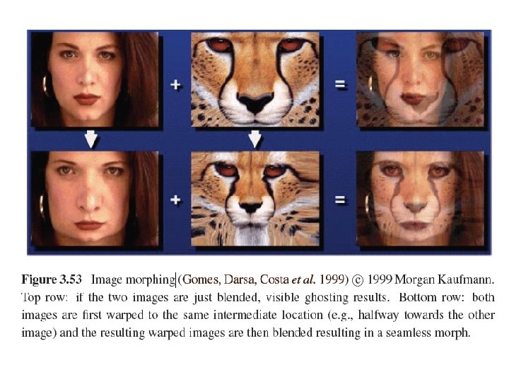
3. 6. 2 Mesh-Based Warping (3/3) 101

102

>0 Control 0. 5 Same weight 0 Same weight Smooth 2 Closer greater 1 Longer lines have greater weight 103

Image Processing • • 3. 1 Point Operators 3. 2 Linear Filtering 3. 3 More Neighborhood Operators 3. 4 Fourier Transforms 3. 5 Pyramids and Wavelets 3. 6 Geometric Transformations 3. 7 Global Optimization 105

3. 7. 1 Regularization (1/6) 106

3. 7. 1 Regularization (2/6) • Finding a smooth surface that passes through (or near) a set of measured data points. • Such a problem is described as ill-posed because many possible surfaces can fit this data. • Since small changes in the input can sometimes lead to large changes in the fit, such problems are also often ill-conditioned. 107

Ill-conditioned System 108

3. 7. 1 Regularization (3/6) • Since we are trying to recover the unknown function f(x, y) from which the data point d(xi, yi) were sampled, such problems are also often called inverse problems. • Many computer vision tasks can be viewed as inverse problems, since we are trying to recover a full description of the 3 D world from a limited set of images. 109

3. 7. 1 Regularization (4/6) • In order to quantify what it means to find a smooth solution, we can define a norm on the solution space. • For one-dimensional functions f(x), we can integrate the squared first derivative of the function, or perhaps integrate the squared second derivative, 110

3. 7. 1 Regularization (5/6) • In two dimensions, the corresponding smoothness functionals are • The first derivative norm is often called the membrane, since interpolating a set of data points using this measure results in a tent-like structure. • The second-order norm is called the thin-plate spline, since it approximates the behavior of thin plates (e. g. , flexible steel) under small deformations. 111

3. 7. 1 Regularization (6/6) • For scattered data interpolation, the data term measures the distance between the function f(x, y) and a set of data points di =d(xi , yi) • To obtain a global energy that can be minimized, the two energy terms are usually added together, : smoothness penalty : regularization parameter 112

Term Project • Tentative term project problems: Exercises in textbook, (30%) total grade: • Submit one page in English explaining method, steps, expected results • Submit report in a month: April 9 • Report progress every other week • All right to be the same problem with Master’s thesis

• Objective: a working prototype with new, original, novel ideas • Objective: not just literature survey • Objective: not just straightforward implementation of existing algorithms • Objective: all right to modify existing algorithms