Advanced Computer Vision Chapter 3 Image Processing 2

Advanced Computer Vision Chapter 3 Image Processing (2) Presented by: 傅楸善 & 張乃婷 0919508863 r 99922068@ntu. edu. tw 1

Image Processing • • 3. 1 Point Operators 3. 2 Linear Filtering 3. 3 More Neighborhood Operators 3. 4 Fourier Transforms 3. 5 Pyramids and Wavelets 3. 6 Geometric Transformations 3. 7 Global Optimization 2

3. 5 Pyramids and Wavelets • Image pyramids are extremely useful for performing multi-scale editing operations such as blending images while maintaining details. • For example, the task of finding a face in an image. Since we do not know the scale at which the face will appear, we need to generate a whole pyramid of differently sized images and scan each one for possible faces. 3

4

3. 5. 1 Interpolation (Upsampling) • Interpolation can be used to increase the resolution of an image. r: upsampling rate. 5

6

Bilinear Interpolation 7

Cubic Interpolation • Bicubic interpolation – Is an extension of cubic interpolation for interpolating data points on a two dimensional regular grid. – The interpolated surface is smoother than corresponding surfaces obtained by bilinear interpolation. 8

9

3. 5. 2 Decimation (Downsampling) • Decimation is required to reduce the resolution. • To perform decimation, we first convolve the image with a low-pass filter (to avoid aliasing) and then keep every rth sample. • h(k, l): smoothing kernel 10

11

3. 5. 3 Multi-Resolution Representations • Pyramids can be used to accelerate coarse-tofine search algorithms, to look for objects or patterns at different scales, and to perform multi-resolution blending operations. • To construct the pyramid, we first blur and subsample the original image by a factor of two and store this in the next level of the pyramid. 12

Gaussian Pyramid (1/2) • The technique involves creating a series of images which are weighted down using a Gaussian average and scaled down. • Five-tap kernel: 13

Gaussian Pyramid (2/2) • The weighting function closely approximates the Gaussian function, hence the origins of the pyramids name. 14

15

Laplacian Pyramid • First, interpolate a lower resolution image to obtain a reconstructed low-pass version of the original image. • They then subtract this low-pass version from the original to yield the band-pass “Laplacian” image, which can be stored away for further processing. 16

Half-Octave pyramids 17

3. 5. 4 Wavelets • Two-dimensional wavelets • The high-pass filter followed by decimation keeps 3/4 of the original pixels, while 1/4 of the low-frequency coefficients are passed on to the next stage for further analysis. • The resulting three wavelet images are called the high –high (HH), high–low (HL), and low–high (LH) images. • The HL and LH images accentuate the horizontal and vertical edges and gradients, while the HH image contains the less frequently occurring mixed 18 derivatives.

19

One-Dimensional Wavelets 20

Lifted Transform 21

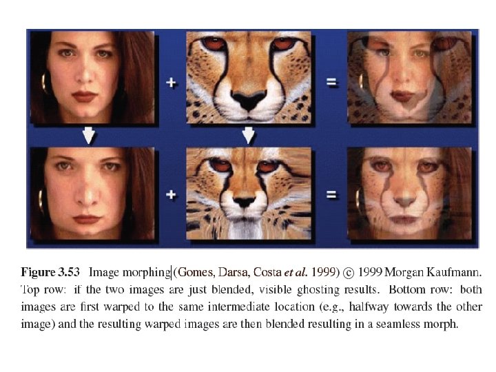
Image Blending 22

23

3. 6 Geometric Transformations 24

3. 6. 1 Parametric Transformations • Parametric transformations apply a global deformation to an image, where the behavior of the transformation is controlled by a small number of parameters. 25

3. 6. 1 Parametric Transformations 26

Forward Warping • The process of copying a pixel f(x) to a location in g is not well defined when has a non-integer value. • You can round the value of to the nearest integer coordinate and copy the pixel there, but the resulting image has severe aliasing and pixels that jump around a lot when animating the transformation. • The second major problem with forward warping is the appearance of cracks and holes, especially when magnifying an image. 27

28

Inverse Warping • is (presumably) defined for all pixels in , we no longer have holes. • it can simply be computed as the inverse of • In fact, all of the parametric transforms listed in Table 3. 5 have closed form solutions for the inverse transform: simply take the inverse of the 3× 3 matrix specifying the transform. 29

30

MIP-Mapping (1/3) • MIP-mapping was first proposed by Williams (1983) as a means to rapidly pre-filter images being used for texture mapping in computer graphics. • A MIP-map is a standard image pyramid, where each level is pre-filtered with a high-quality filter rather than a poorer quality approximation, such as five-tap binomial. 31

MIP-Mapping (2/3) • To resample an image from a MIP-map, a scalar estimate of the resampling rate r is first computed. • For example, r can be the maximum of the absolute values in A (which suppresses aliasing) or it can be the minimum (which reduces blurring). • Once a resampling rate has been specified, a fractional pyramid level is computed using the base 2 logarithm, 32

MIP-Mapping (3/3) • One simple solution is to resample the texture from the next higher or lower pyramid level, depending on whether it is preferable to reduce aliasing or blur. • Since most MIP-map implementations use bilinear resampling within each level, this approach is usually called trilinear MIP-mapping. 33

34

Elliptical Weighted Average (EWA) • The Elliptical Weighted Average filter is based on the observation that the affine mapping defines a skewed two-dimensional coordinate system in the vicinity of each source pixel x. • For every destination pixel , the ellipsoidal projection of a small pixel grid in onto x is computed. • This is used to filter the source image g(x) with a Gaussian whose inverse covariance matrix is ellipsoid. 35

Anisotropic Filtering • In this approach, several samples at different resolutions (fractional levels in the MIP-map) are combined along the major axis of the EWA Gaussian. 36

Multi-Pass Transforms (1/3) • The optimal approach to warping images without excessive blurring or aliasing is to adaptively pre-filter the source image at each pixel using an ideal low-pass filter, i. e. , an oriented skewed sinc or low-order (e. g. , cubic) approximation. 37

Multi-Pass Transforms (2/3) 38

Multi-Pass Transforms (3/3) • For parametric transforms, the oriented twodimensional filtering and resampling operations can be approximated using a series of one-dimensional resampling and shearing transforms. • In order to prevent aliasing, however, it may be necessary to upsample in the opposite direction before applying a shearing transformation. 39

40

3. 6. 2 Mesh-Based Warping (1/3) • While parametric transforms specified by a small number of global parameters have many uses, local deformations with more degrees of freedom are often required. • Different amounts of motion are required in different parts of the image. 41

3. 6. 2 Mesh-Based Warping (2/3) 42

3. 6. 2 Mesh-Based Warping (3/3) • The first approach, is to specify a sparse set of corresponding points. The displacement of these points can then be interpolated to a dense displacement field. • A second approach to specifying displacements for local deformations is to use corresponding oriented line segments. 43

3. 7 Global Optimization • Regularization (variational methods) – Constructs a continuous global energy function that describes the desired characteristics of the solution and then finds a minimum energy solution using sparse linear systems or related iterative techniques. • Markov random field – Using Bayesian statistics, modeling both the noisy measurement process that produced the input images as well as prior assumptions about the solution space. 45

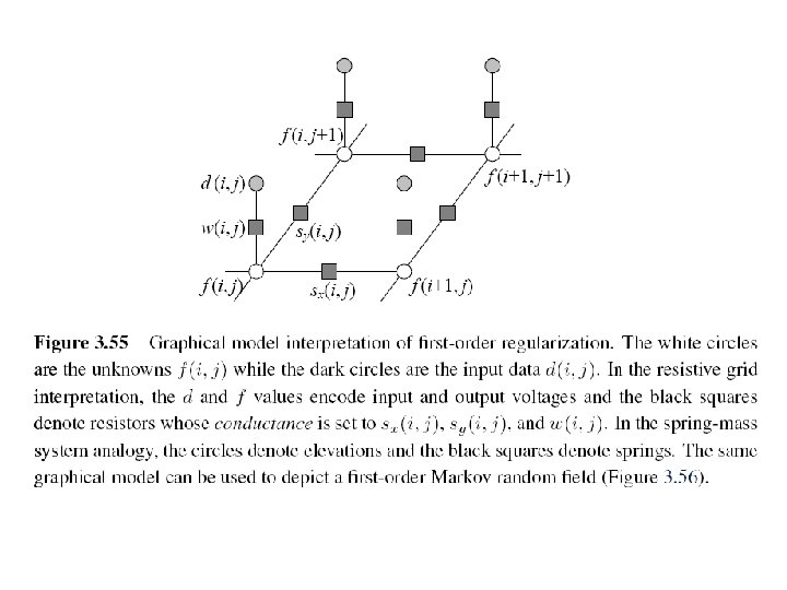
3. 7. 1 Regularization (1/6) 46

3. 7. 1 Regularization (2/6) • Finding a smooth surface that passes through (or near) a set of measured data points. • Such a problem is described as because illposed many possible surfaces can fit this data. • Since small changes in the input can sometimes lead to large changes in the fit, such problems are also often ill-conditioned. 47

3. 7. 1 Regularization (3/6) • Since we are trying to recover the unknown function f(x, y) from which the data point d(xi, yi) were sampled, such problems are also often called inverse problems. • Many computer vision tasks can be viewed as inverse problems, since we are trying to recover a full description of the 3 D world from a limited set of images. 48

3. 7. 1 Regularization (4/6) • In order to quantify what it means to find a smooth solution, we can define a norm on the solution space. • For one-dimensional functions f(x), we can integrate the squared first derivative of the function, or perhaps integrate the squared second derivative, 49

3. 7. 1 Regularization (5/6) • In two dimensions, the corresponding smoothness functionals are • The first derivative norm is often called the membrane, since interpolating a set of data points using this measure results in a tent-like structure. • The second-order norm is called the thin-plate spline, since it approximates the behavior of thin plates (e. g. , flexible steel) under small deformations. 50

3. 7. 1 Regularization (6/6) • For scattered data interpolation, the data term measures the distance between the function f(x, y) and a set of data points di =d(xi , yi) • To obtain a global energy that can be minimized, the two energy terms are usually added together, 51

3. 7. 2 Markov Random Fields (1/3) • The posterior distribution for a given set of measurements y, combined with a prior p(x) over the unknowns x, is given by • Negative posterior log likelihood. 53

3. 7. 2 Markov Random Fields (2/3) • To find the most likely (maximum a posteriori or MAP) solution x given some measurements y, we simply minimize this negative log likelihood, which can also be thought of as an energy, • Ed(x, y) is the data energy or data penalty • Ep(x) is the prior energy

3. 7. 2 Markov Random Fields (3/3) • For image processing applications, the unknowns x are the set of output pixels • The data are (in the simplest case) the input pixels

56

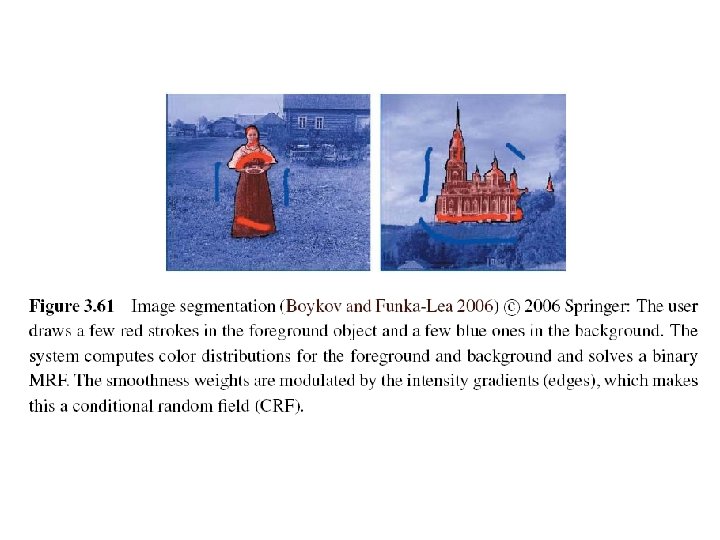
Binary MRFs • The simplest possible example of a Markov random field is a binary field. • Examples of such fields include 1 -bit (black and white) scanned document images as well as images segmented into foreground and background regions.

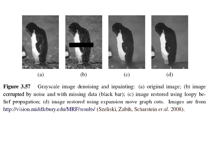
Ordinal-Valued MRFs • In addition to binary images, Markov random fields can be applied to ordinal-valued labels such as grayscale images or depth maps. • The term “ordinal” indicates that the labels have an implied ordering, e. g. , that higher values are lighter pixels.

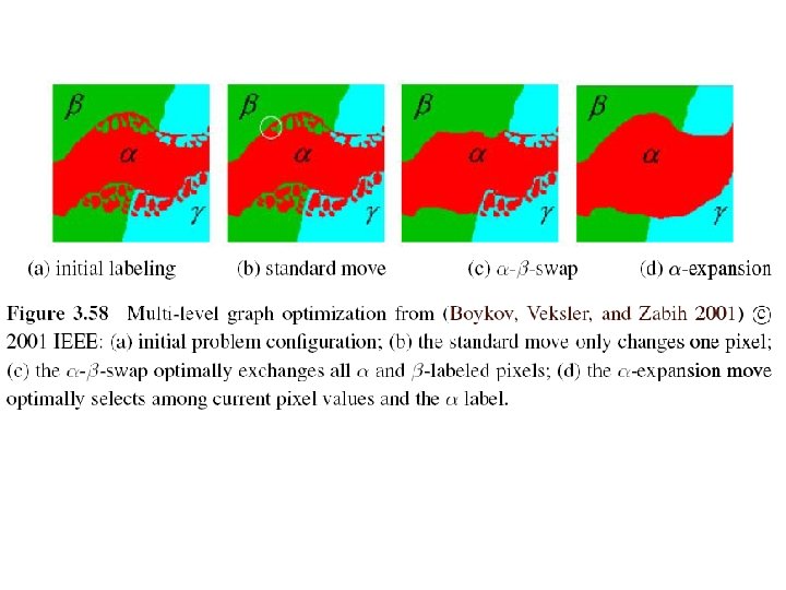
Unordered Labels

Term Project • Tentative term project problems: Exercises in textbook, (30%) total grade: • Submit one page in English explaining method, steps, expected results • Submit report in a month: April 12 • Report progress every other week • All right to be the same problem with Master’s thesis

• Objective: a working prototype with new, original, novel ideas • Objective: not just literature survey • Objective: not just straightforward implementation of existing algorithms • Objective: all right to modify existing algorithms