A suite of Stata programs for network metaanalysis

A suite of Stata programs for network meta-analysis UK Stata users’ Group London, 13 th September 2013 Ian White MRC Biostatistics Unit, Cambridge, UK

Plan • Ordinary (pairwise) meta-analysis • Multiple treatments: indirect comparisons, consistency, inconsistency • Network meta-analysis: models • Fitting network meta-analysis: Win. BUGS and Stata • Data formats • network: its aims and scope; fitting models in different formats; graphical displays • My difficulties 2

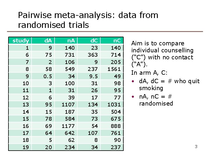
Pairwise meta-analysis: data from randomised trials study 1 6 7 8 9 10 11 12 13 14 15 16 17 18 19 d. A 9 75 2 58 0. 5 3 1 6 95 15 78 69 64 5 20 n. A 140 731 106 549 34 100 31 39 1107 187 584 1177 642 62 234 d. C 23 363 9 237 9. 5 31 26 17 134 35 73 54 107 8 34 n. C 140 714 205 1561 49 98 95 77 1031 504 675 888 761 90 237 Aim is to compare individual counselling (“C”) with no contact (“A”). In arm A, C: • d. A, d. C = # who quit smoking • n. A, n. C = # randomised 3

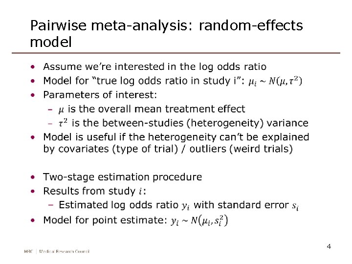
Pairwise meta-analysis: random-effects model • 4

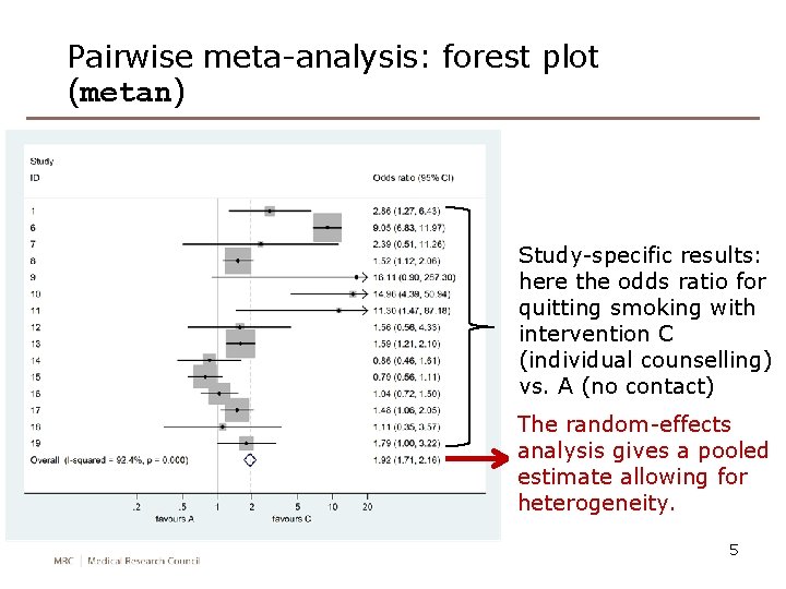
Pairwise meta-analysis: forest plot (metan) Study-specific results: here the odds ratio for quitting smoking with intervention C (individual counselling) vs. A (no contact) The random-effects analysis gives a pooled estimate allowing for heterogeneity. 5

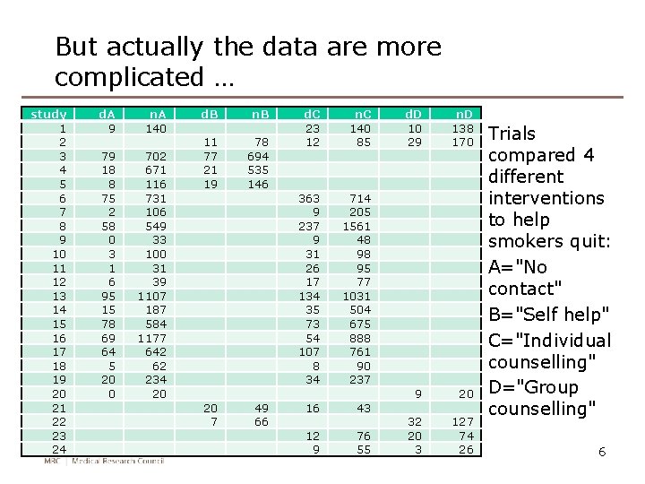
But actually the data are more complicated … study 1 2 3 4 5 6 7 8 9 10 11 12 13 14 15 16 17 18 19 20 21 22 23 24 d. A 9 n. A 140 79 18 8 75 2 58 0 3 1 6 95 15 78 69 64 5 20 0 702 671 116 731 106 549 33 100 31 39 1107 187 584 1177 642 62 234 20 d. B n. B 11 77 21 19 78 694 535 146 20 7 49 66 d. C 23 12 n. C 140 85 363 9 237 9 31 26 17 134 35 73 54 107 8 34 714 205 1561 48 98 95 77 1031 504 675 888 761 90 237 16 43 12 9 76 55 d. D 10 29 n. D 138 170 9 20 32 20 3 127 74 26 Trials compared 4 different interventions to help smokers quit: A="No contact" B="Self help" C="Individual counselling" D="Group counselling" 6

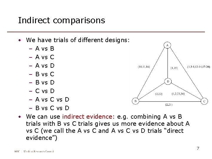
Indirect comparisons • We have trials of different designs: – A vs B – A vs C – A vs D – B vs C – B vs D – C vs D – A vs C vs D – B vs C vs D • We can use indirect evidence: e. g. combining A vs B trials with B vs C trials gives us more evidence about A vs C (we call the A vs C and A vs C vs D trials “direct evidence”) 7

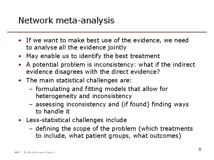
Network meta-analysis • If we want to make best use of the evidence, we need to analyse all the evidence jointly • May enable us to identify the best treatment • A potential problem is inconsistency: what if the indirect evidence disagrees with the direct evidence? • The main statistical challenges are: – formulating and fitting models that allow for heterogeneity and inconsistency – assessing inconsistency and (if found) finding ways to handle it • Less-statistical challenges include – defining the scope of the problem (which treatments to include, what patient groups, what outcomes) 8

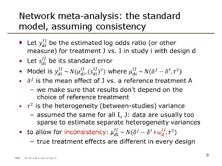
Network meta-analysis: the standard model, assuming consistency • 9

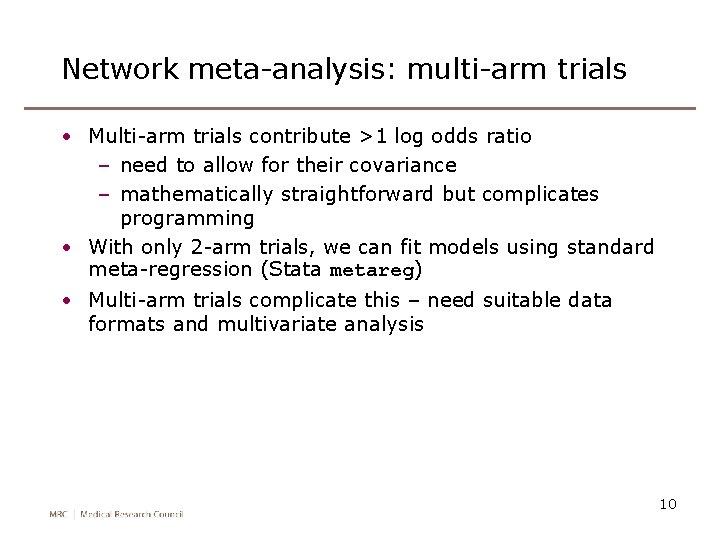
Network meta-analysis: multi-arm trials • Multi-arm trials contribute >1 log odds ratio – need to allow for their covariance – mathematically straightforward but complicates programming • With only 2 -arm trials, we can fit models using standard meta-regression (Stata metareg) • Multi-arm trials complicate this – need suitable data formats and multivariate analysis 10

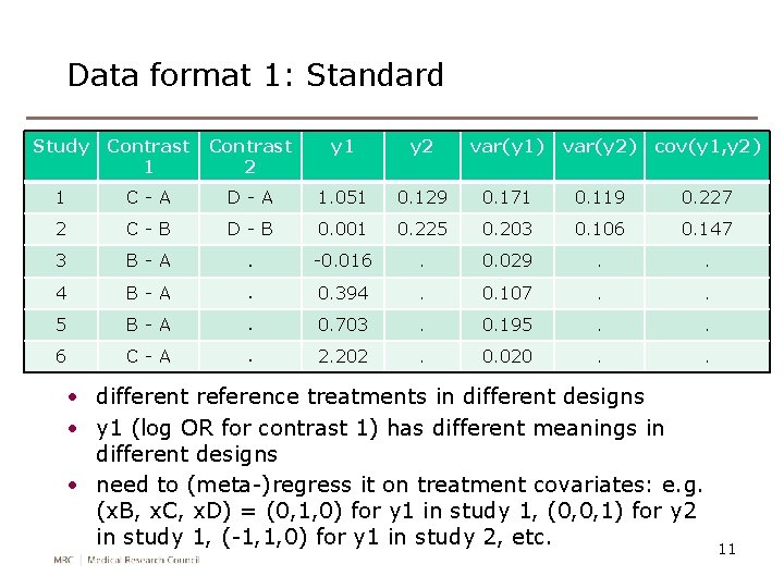
Data format 1: Standard Study Contrast 1 Contrast 2 y 1 y 2 var(y 1) var(y 2) cov(y 1, y 2) 1 C - A D - A 1. 051 0. 129 0. 171 0. 119 0. 227 2 C - B D - B 0. 001 0. 225 0. 203 0. 106 0. 147 3 B - A . -0. 016 . 0. 029 . . 4 B - A . 0. 394 . 0. 107 . . 5 B - A . 0. 703 . 0. 195 . . 6 C - A . 2. 202 . 0. 020 . . • different reference treatments in different designs • y 1 (log OR for contrast 1) has different meanings in different designs • need to (meta-)regress it on treatment covariates: e. g. (x. B, x. C, x. D) = (0, 1, 0) for y 1 in study 1, (0, 0, 1) for y 2 in study 1, (-1, 1, 0) for y 1 in study 2, etc. 11

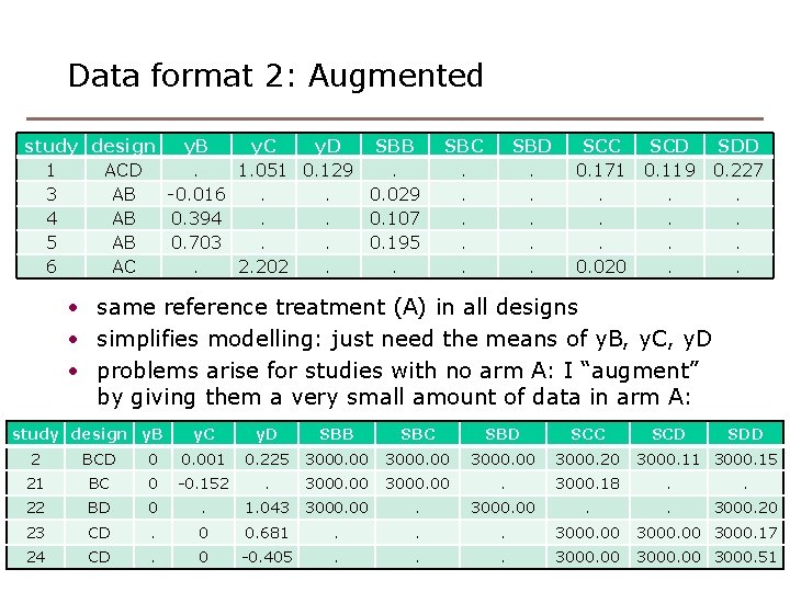
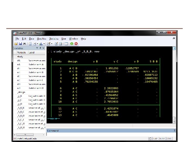
Data format 2: Augmented study design y. B y. C y. D SBB 1 ACD. 1. 051 0. 129. 3 AB -0. 016. . 0. 029 4 AB 0. 394. . 0. 107 5 AB 0. 703. . 0. 195 6 AC. 2. 202. . SBC. . . SBD. . . SCC 0. 171. . . 0. 020 SCD 0. 119. . SDD 0. 227. . • same reference treatment (A) in all designs • simplifies modelling: just need the means of y. B, y. C, y. D • problems arise for studies with no arm A: I “augment” by giving them a very small amount of data in arm A: study design y. B y. C y. D SBB SBC SBD SCC SCD SDD 2 BCD 0 0. 001 0. 225 3000. 00 3000. 20 3000. 11 3000. 15 21 BC 0 -0. 152 . 3000. 00 . 3000. 18 . . 22 BD 0 . 1. 043 3000. 00 . . 3000. 20 23 CD . 0 0. 681 . . . 3000. 00 24 CD . 0 -0. 405 . . . 3000. 00 3000. 17 12 3000. 00 3000. 51

Fitting network meta-analyses • In the past, the models have been fitted using Win. BUGS – because frequentist alternatives have not been available – has made network meta-analysis inaccessible to nonstatisticians • Now, consistency and inconsistency models can be fitted for both data formats using multivariate meta-analysis or multivariate meta-regression – using my mvmeta • Parameterising the consistency model for “augmented” format is easy • Allowing for inconsistency and “standard” format is trickier … 13

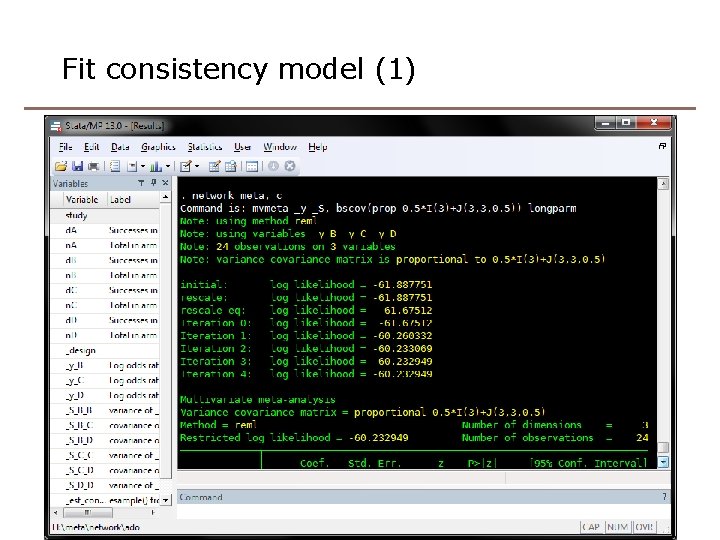
Aims of the network suite • Automatically convert network data to the correct format for multivariate meta-analysis • Automatically set up mvmeta models for consistency and inconsistency, and run them • Provide graphical displays to aid understanding of data and results • Handle both standard and augmented formats, and convert between them, in order to demonstrate their equivalence • Interface with other Stata software for network metaanalysis 14

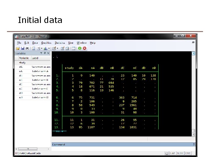
Initial data 15

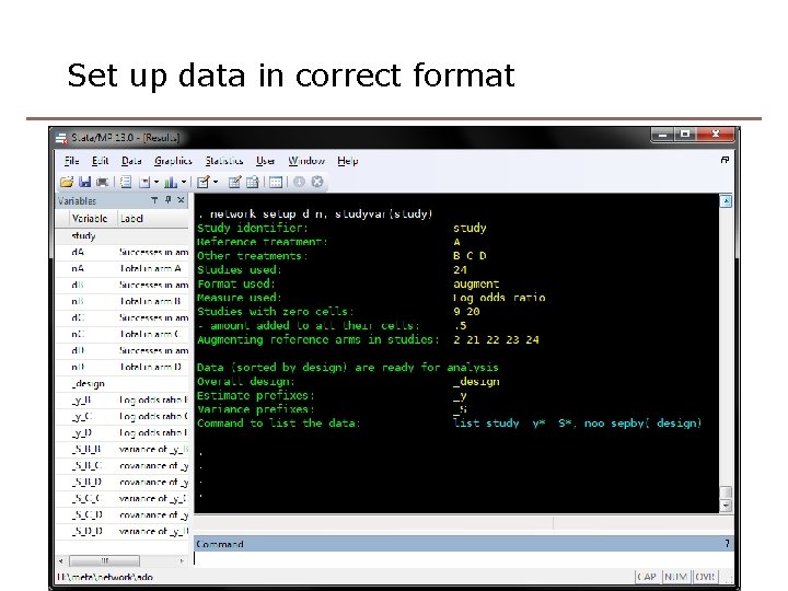
Set up data in correct format 16

17

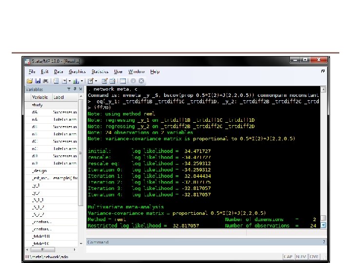
Fit consistency model (1) 18

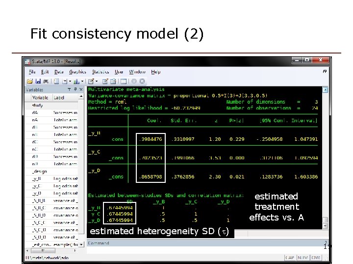
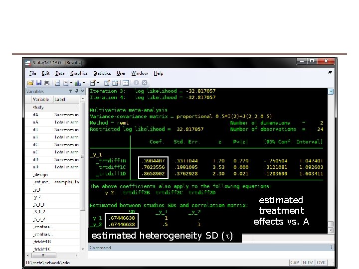
Fit consistency model (2) estimated treatment effects vs. A estimated heterogeneity SD (t) 19

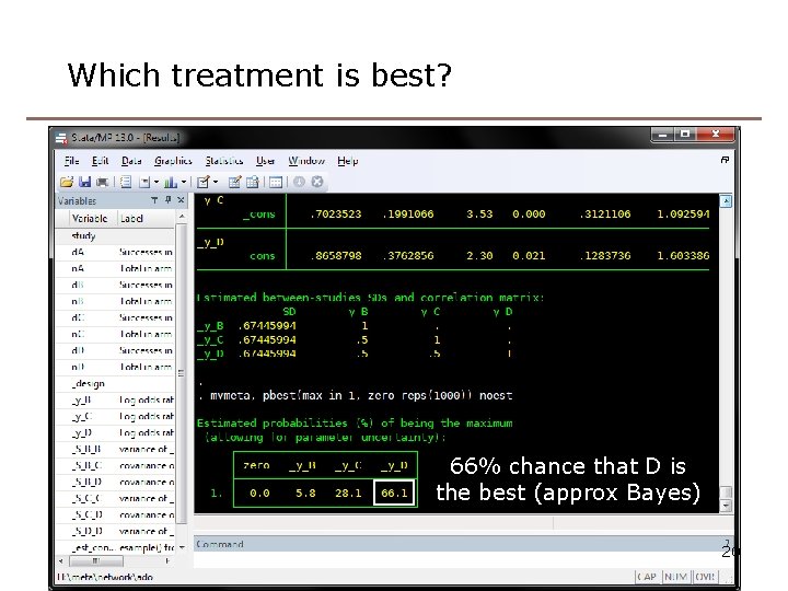
Which treatment is best? 66% chance that D is the best (approx Bayes) 20

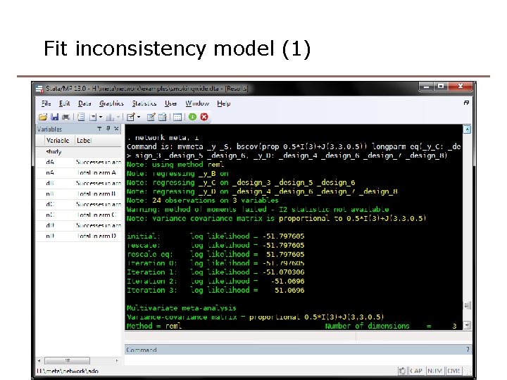
Fit inconsistency model (1) 21

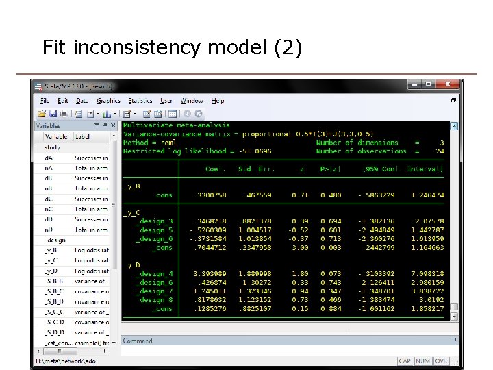
Fit inconsistency model (2) 22

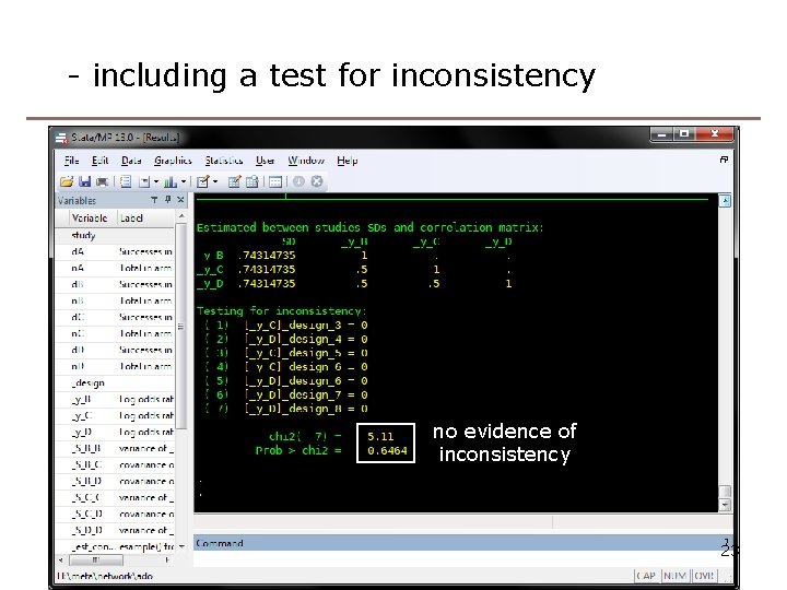
- including a test for inconsistency no evidence of inconsistency 23

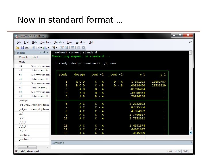
Now in standard format … 24

25

estimated treatment effects vs. A estimated heterogeneity SD (t) 26

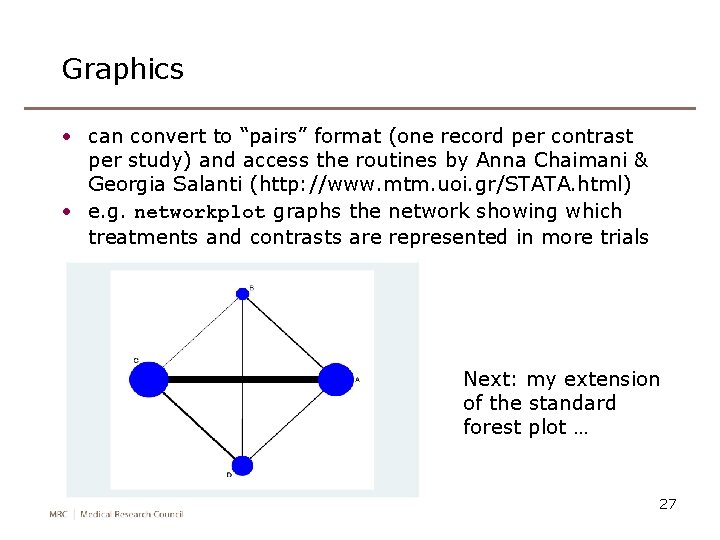
Graphics • can convert to “pairs” format (one record per contrast per study) and access the routines by Anna Chaimani & Georgia Salanti (http: //www. mtm. uoi. gr/STATA. html) • e. g. networkplot graphs the network showing which treatments and contrasts are represented in more trials Next: my extension of the standard forest plot … 27

28

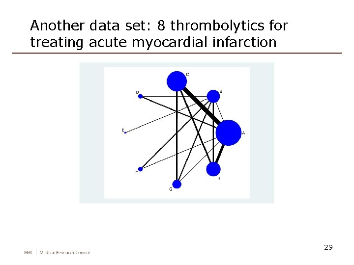
Another data set: 8 thrombolytics for treating acute myocardial infarction 29

30

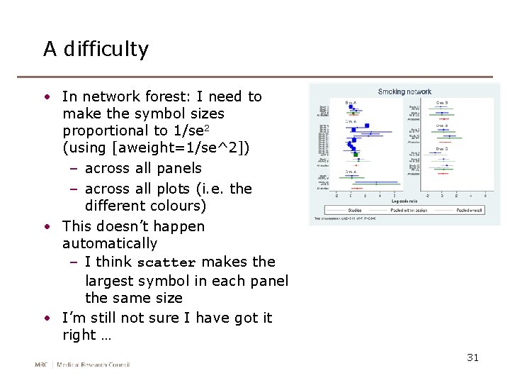
A difficulty • In network forest: I need to make the symbol sizes proportional to 1/se 2 (using [aweight=1/se^2]) – across all panels – across all plots (i. e. the different colours) • This doesn’t happen automatically – I think scatter makes the largest symbol in each panel the same size • I’m still not sure I have got it right … 31

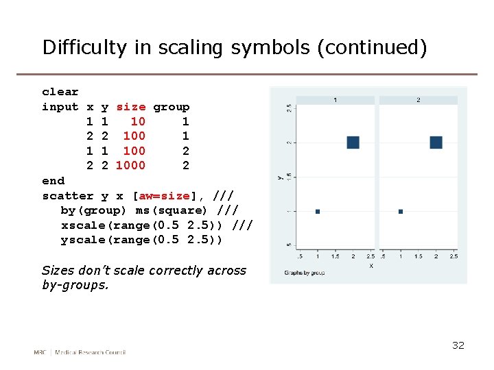
Difficulty in scaling symbols (continued) clear input x y size group 1 1 10 1 2 2 100 1 100 2 2 2 1000 2 end scatter y x [aw=size], /// by(group) ms(square) /// xscale(range(0. 5 2. 5)) /// yscale(range(0. 5 2. 5)) Sizes don’t scale correctly across by-groups. 32

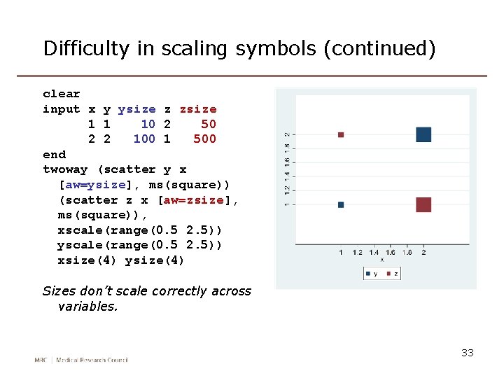
Difficulty in scaling symbols (continued) clear input x y ysize z zsize 1 1 10 2 50 2 2 100 1 500 end twoway (scatter y x [aw=ysize], ms(square)) (scatter z x [aw=zsize], ms(square)), xscale(range(0. 5 2. 5)) yscale(range(0. 5 2. 5)) xsize(4) ysize(4) Sizes don’t scale correctly across variables. 33

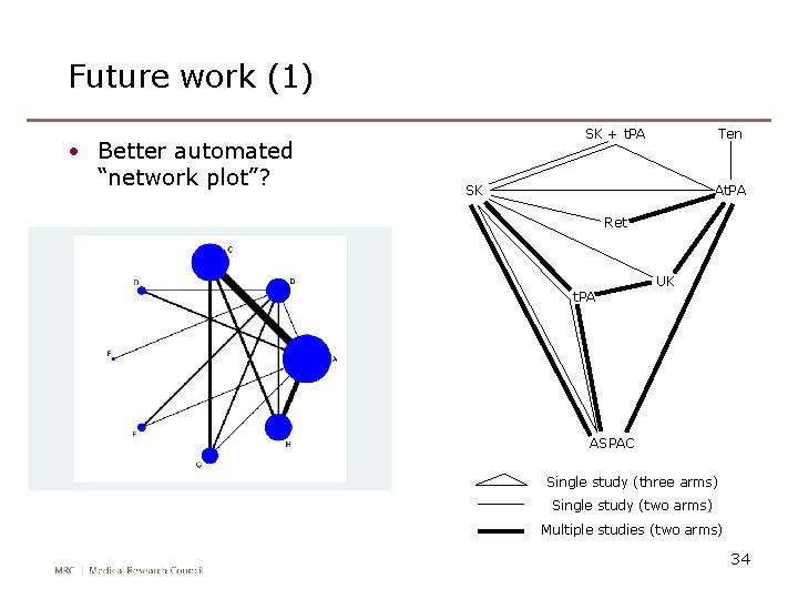
Future work (1) • Better automated “network plot”? Ten SK + t. PA SK At. PA Ret t. PA UK ASPAC Single study (three arms) Single study (two arms) Multiple studies (two arms) 34

Future work (2) • Release to users • Allow more complex variance structures for the heterogeneity terms • Random inconsistency model Thanks to Julian Higgins, Dan Jackson and Jessica Barrett who worked with me on this. Key references: • Lu G, Ades AE. Assessing evidence inconsistency in mixed treatment comparisons. Journal of the American Statistical Association 2006; 101: 447– 459. • White IR, Barrett JK, Jackson D, Higgins JPT. Consistency and inconsistency in network meta-analysis: model estimation using multivariate meta-regression. Research Synthesis Methods 2012; 3: 111– 125. 35

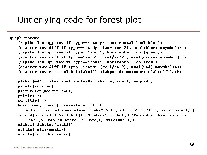
Underlying code forest plot graph twoway (rspike low upp row if type=="study", horizontal lcol(blue)) (scatter row diff if type=="study" [aw=1/se^2], mcol(blue) msymbol(S)) (rspike low upp row if type=="inco", horizontal lcol(green)) (scatter row diff if type=="inco" [aw=1/se^2], mcol(green) msymbol(S)) (rspike low upp row if type=="cons", horizontal lcol(red)) (scatter row diff if type=="cons" [aw=1/se^2], mcol(red) msymbol(S)) (scatter row zero, mlabel(label 2) mlabpos(0) ms(none) mlabcol(black)) , ylabel(#44, valuelabel angle(0) labsize(vsmall) nogrid ) yscale(reverse) plotregion(margin(t=0)) ytitle("") subtitle("") by(column, row(1) yrescale noiytick note(`"Test of consistency: chi 2=5. 11, df=7, P=0. 646"', size(vsmall))) legend(order(1 3 5) label(1 "Studies") label(3 "Pooled within design") label(5 "Pooled overall") row(1) size(small)) xlabel(, labsize(small)) xtitle(, size(small)) xtitle(Log odds ratio) ; 36