2 Time Independent Schrodinger Equation 1 Stationary States

2. Time Independent Schrodinger Equation 1. Stationary States 2. The Infinite Square Well 3. The Harmonic Oscillator 4. The Free Particle 5. The Delta Function Potential 6. The Finite Square Well

1. 1. Stationary States Schrodinger Equation : Assume ( is separable ) = const = E if V = V(r) Time-independent Schrodinger eq.

Properties of Separable 1. Stationary States: Expectation values are time-independent. In particular :

2. Definite E : Hamiltonian : Time-independent Schrodinger eq. becomes

3. Expands Any General Solution : Any general solution of the time dependent Schrodinger eq. can be written as where The cn s are determined from { n } is complete. Proof :

Example 2. 1 A particle starts out as What is ( x, t ) ? Find the probability, and describe its motion. Ans. if c & are real. Read Prob 2. 1, 2. 2

2. The Infinite Square Well 0 for x [ 0, a ] General solution. Allowable boundary conditions ( for 2 nd order differential eqs ) : and can both be continuous at a regular point (i. e. where V is finite). Only can be continuous at a singular point (i. e. where V is infinite).

Boundary Conditions B. C. : continuous at x = 0 and a , i. e. , n = 0 0 (not physically meaningful). k give the same independent solution. E is quantized. Normalization:

Eigenstates with B. C. has a set of normalized eigenfunctions with eigenvalues n = 1 is the ground (lowest energy) state. All other states with n > 1 are excited states. even, 0 node. odd, 1 node. even, 2 nodes.

Properties of the Eigenstates 1. Parity = ( ) n 1. [ True for any symmetric V ] 2. Number of nodes n 1. [ Universal ] 3. Orthogonality: [ Universal ] if m n. Orthonormality: 4. Completeness: [ Universal ] Any function f on the same domain and with the same boundary conditions as the n s can be written as

Proof of Orthonormality

Condition for Completeness where { n } is orthonormal. Let Then if { n } is complete.

Conclusion Stationary state of energy General solution: where so that is

Example 2. 2 A particle in an infinite well has initial wave function Find ( x, t ). Ans. Using we have

Normalization: for n odd B = Bernoulli numbers

In general : { n } orthonormal normalized If then | cn |2 = probability of particle in state n. H average of En weighted by the occupation probability.

Example 2. 3. In Example 2. 2, ( x, t ) closely resembles 1 (x) , which suggests | c 1 |2 should dominate. Indeed, where Do Prob 2. 8, 2. 9

3. The Harmonic Oscillator Classical Mechanics: Hooke’s law: Newton’s 2 nd law. Solution: Potential energy: parabolic Any potential is parabolic near a local minimum. where

Quantum Mechanics: Schrodinger eq. : Methods for solution: 1. Power series ( analytic ) Hermite functions. 2. Number space (algebraic) a , a+ operators.

3. 1. Algebraic Method Schrodinger eq. in operator form: Commutator of operators A and B : f Eg. Let canonical commutation relation , real, positive constants

Set Let i. e. , H , a+a and a a+ all share the same eigenstates. Their eigenvalues are related by where

Adjoint or Hermitian Conjugate of an Operator Given an operator A , its adjoint (Hermitian conjugate) A+ is defined by , , real & positive Proof : ( , 0 at boundaries ) Integration by part gives: Note:

n-Representation Consider an operator a with the property Define the operator with its eigenstates and eigenvalues Meaning of a+ n : a+ n is an eigenstate with eigenvalue larger than that of n by 1. a+ raising op Meaning of a n : a n is an eigenstate with eigenvalue smaller than that of n by 1. Let N be bounded below ( there is a ground state 0 with eigenvalue 0 ). i. e. Hence with a lowering op

Normalization ( , normalization const. ) Let with Assuming , real : n

Orthonormality for m n

Harmonic Oscillator : n-Representation a ~ a , a+ ~ a+ , Equation for 0 : a+ a ~ a+ a

0 Set A real : Normalized

Example 2. 4 Find the first excited state of the harmonic oscillator. Ans:

Example 2. 5 Find V for the nth state of the harmonic oscillator. Ans: Do Prob 2. 13

3. 2. Analytic Method is solved analytically. Set where

Asymptotic Form For x, as Set normalizable h solved by Frobenius method (power series expansion)

h( ) Asume recursion formula

Termination Even & odd series starting with a 0 & a 1 , resp. For large j : explodes as Power series must terminate. Set j n+2

with E En

Hermite Polynomials Hermite polynomials : n even : set a 0 1 , a 1 0 n odd : set a 0 0 , a 1 1 an 2 n Normalized :

n n 3 n 2 n 1 n 0

| 100 |2 , (x) Classical distribution : A = amplitude Do Prob 2. 15, 2. 16 Read Prob 2. 17

4. The Free Particle Eigenstate: Stationary state: to right to left Reset: k > 0 : to right k < 0 : to left phase velocity

Oddities about k (x, t) Classical mechanics : not normalizable k is not physical (cannot be truly realized physically ). k is a mathematical solution ( can be used to expand a physical state or as an idealization ).

Wave Packets General free particle state : wave packet Fourier transform

Example 2. 6 A free particle, initially localized within [ a, a ], is released at t 0 : A, a real & positive Find ( x, t ). Ans: Normalize ( x, 0 ) :

t=0 FT of Gaussian is a Gaussian.

Group Velocity (k) = dispersion In general : For a well defined wave packet, is narrowly peaked at some k = k 0. To calculate ( x, t ), one need only ( moves with velocity 0 . ) 3 -D Define group velocity Free particle wave packet : Reminder: phase velocity Do Prob 2. 19 Read Prob 2. 20

Example 2. 6 A Consider a free particle wave packet with (k) given by A, a real & positive Find ( x, t ). Ans: Normalize ( x, 0 ) :

t = { 0, 1, 2 }ma 2/

5. The Delta Function Potential 1. Bound States & Scattering States 2. The Delta Function Well

5. 1. Bound States & Scattering States Classical turning points x 0 : If V(r) E for r D and V(r) > E for r D, then the system is in a bound state for r D. If V(r) E everywhere, then the system is in a scattering state. Quantum systems (w / tunneling) : If V( ) > E, then the system is in a bound state. If V( ) < E, then the system is in a scattering state. If V( ) = 0, then E < 0 bound state. E > 0 scattering state.

The Delta Function Dirac delta function : such that f , a, and c > b is a generalized function ( a distribution). [ To be used ONLY inside integrals. ] Setting f (x) = 1 gives Rule : Proof : ( meaningful only inside integrals. )

2. The Delta Function Well For x 0 : Bound states : E<0 Scattering states : E>0 Boundary conditions : 1. continuous everywhere. 2. continuous wherever V is finite.

Bound States For x 0 : Bound states ( E < 0 ) : Set real & positive ( ) = 0 continuous at x 0 B C

Discontinuity in (x 0) is discontinuous at V(x 0) . Let continuous & finite

Only one bound state Normalization :

Scattering States Scattering states ( E > 0 ) : Set for x 0 k real & positive continuous at x 0 Let

2 eqs. , 4 unknown, no normalization. Scattering from left : x Reflection coefficient Transmission coefficient A : incident wave B : reflected wave C : transmitted wave D=0

Delta Function Barrier No bound states For the scattering states, results can be obtained from those of the delta function well by setting . Note: Since E < V inside the barrier, T 0 is called quantum tunneling. ( T = 0 in CM) Also: In QM, R 0 even if E > Vmax. ( R = 0 in CM) Do Prob 2. 24 Read Prob 2. 26

6. The Finite Square Well

Bound States ( E < 0 ) l & are real & positive finite Symmetry : If (x) is a solution, ( x) is also a solution.

Even Solutions continuous at a : or where or

Graphic Solutions E<0 z < z 0

Limiting Cases 1. Wide, deep well ( z 0 large ) : Lower solutions : c. f. infinite well 2. Shallow, narrow well ( z 0 < / 2 ) : Always 1 bound state.

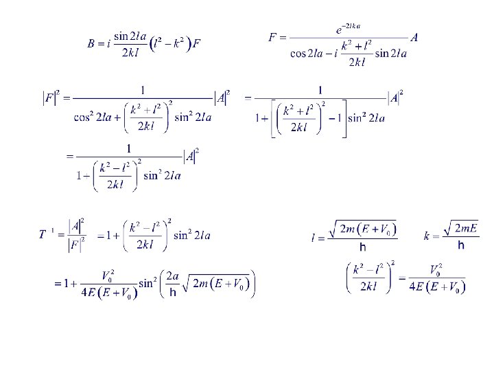
Scattering States ( E > 0 ) l & k are real & positive

Scattering from the Left continuous at a : continuous at a : Eliminate C, D and express B , F in terms of A ( Prob 2. 32 ) :

T 1 when ( well transparent ) i. e. ( at energies of infinite well ) ( Ramsauer-Townsend Effect ) Do Prob 2. 34