Solving the radial Schrdinger equation of hydrogen atom

Solving the radial Schrödinger equation of hydrogen atom for l =0 Yoon Tiem Leong Presentation at the Weekly coffee meeting, Theory Group School of Physics, USM 21 Nov 2008

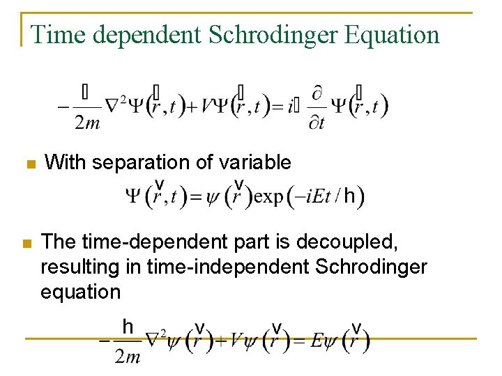
Time dependent Schrodinger Equation n n With separation of variable The time-dependent part is decoupled, resulting in time-independent Schrodinger equation

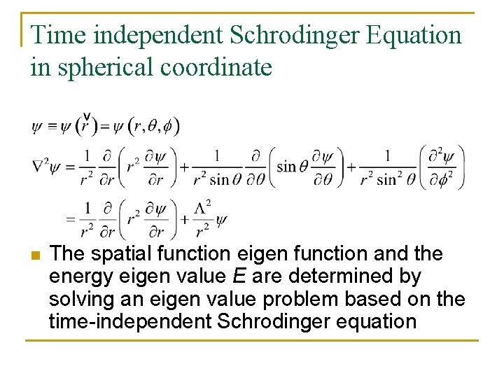
Time independent Schrodinger Equation in spherical coordinate n The spatial function eigen function and the energy eigen value E are determined by solving an eigen value problem based on the time-independent Schrodinger equation

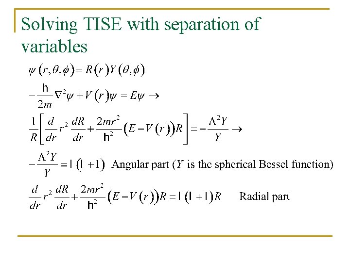
Solving TISE with separation of variables

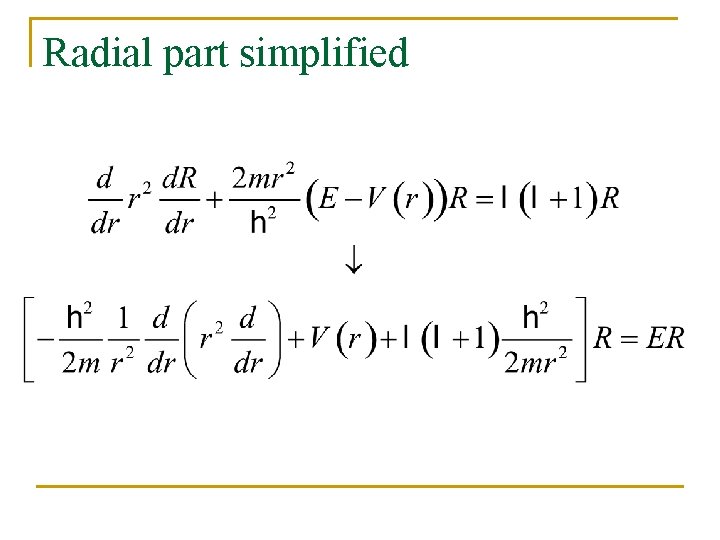
Radial part simplified

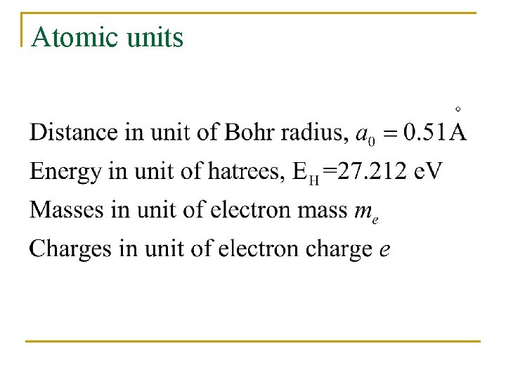
Atomic units

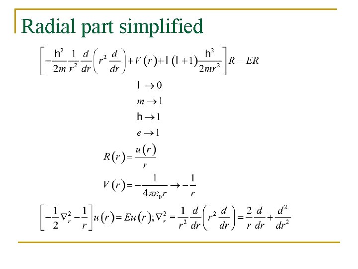
Radial part simplified

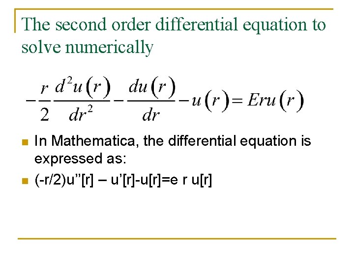
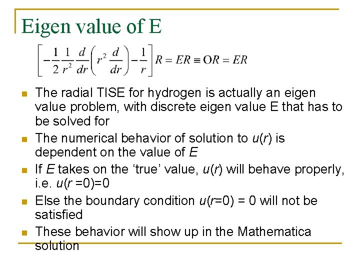
The second order differential equation to solve numerically n n In Mathematica, the differential equation is expressed as: (-r/2)u’’[r] – u’[r]-u[r]=e r u[r]

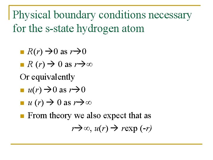
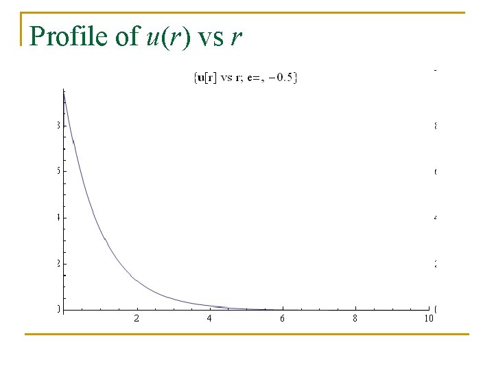
Physical boundary conditions necessary for the s-state hydrogen atom R(r) 0 as r 0 n R (r) 0 as r ∞ Or equivalently n u(r) 0 as r 0 n u (r) 0 as r ∞ n From theory we also expect that as r ∞, u(r) rexp (-r) n

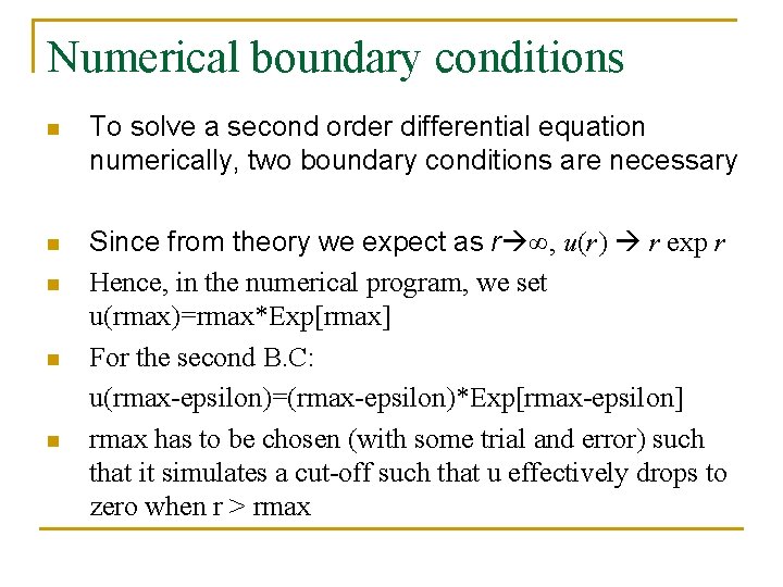
Numerical boundary conditions n To solve a second order differential equation numerically, two boundary conditions are necessary n Since from theory we expect as r ∞, u(r) r exp r Hence, in the numerical program, we set u(rmax)=rmax*Exp[rmax] For the second B. C: u(rmax-epsilon)=(rmax-epsilon)*Exp[rmax-epsilon] rmax has to be chosen (with some trial and error) such that it simulates a cut-off such that u effectively drops to zero when r > rmax n n n

Eigen value of E n n n The radial TISE for hydrogen is actually an eigen value problem, with discrete eigen value E that has to be solved for The numerical behavior of solution to u(r) is dependent on the value of E If E takes on the ‘true’ value, u(r) will behave properly, i. e. u(r =0)=0 Else the boundary condition u(r=0) = 0 will not be satisfied These behavior will show up in the Mathematica solution

NDSolve command line n n n n sol[n_]: =NDSolve[ {-1 u'[r]-r/2 u''[r]-u[r]==r e[n]u[r], u[rmax]==rmax*Exp[-rmax], u[rmax-epsilon]==(rmax-epsilon)*Exp[-(rmaxepsilon)]}, u, {r, epsilon/5, rmax} ] Note that the range cannot be starting from r = 0 but only at r ~ epsilon, or else the numerical code will not work due to computational artifact effect

Input values n n n n e[n]=eguess + n*epsilon Input values: nlow=-410500; nup=-390000; eguess=-0. 1 Epsilon= N[10^(-6)] tol=N[10^(-5)] determine the accuracy of the calculation

NDSolve with a trial E = e[n] n n n n The radial equation (-r/2)u’’[r] – u’[r]-u[r]=e r u[r] is solved with boundary conditions u(rmax)=rmax*Exp[rmax] u(rmax-epsilon)=(rmax-epsilon)*Exp[rmax-epsilon] with a trial value of e[n]=eguess + n*epsilon The energy E = e[n], is parametrised in terms of n The result is a list of numerical values of u[r] as a function of r from r=epsilon to r=rmax

The zero of u[0] n n n Once the numerical solution of u[r] is obtained we can the check the value of u[0] correspond to the value of e[n] = eguess + n*epsilon u[0] is energy-dependent (controlled by n) We then plot a graph of u[0] versus n to locate the interval of n within which the zero of u[0] occur To investigate the zero of u[0] we have to tell the program the range of n, nlow, nup. Have to choose nlow, nup wisely

Root finding n n It should occur around n~400, 000, corresponds to e[n]=eguess+epsilon*n What is the exact value n with u[0] zero?

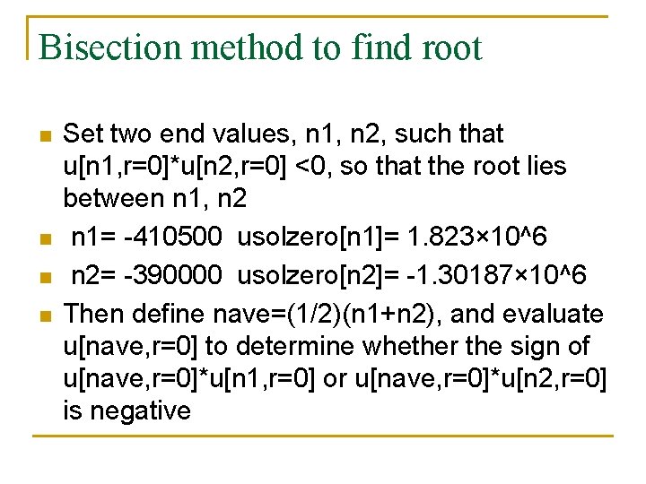
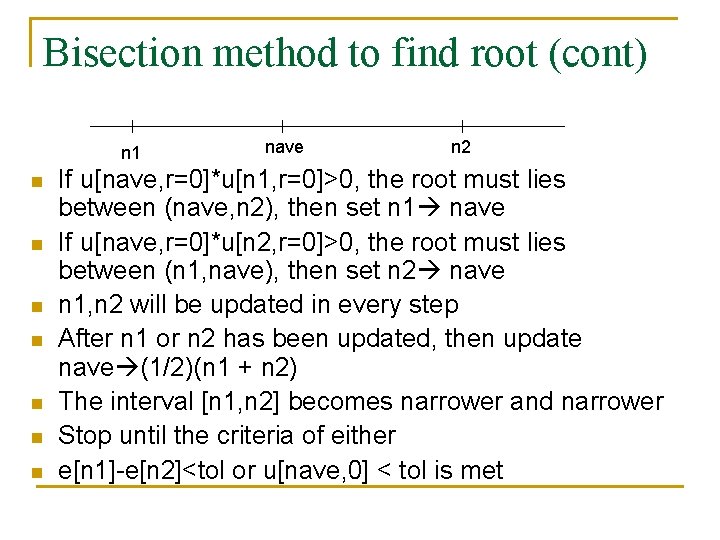
Bisection method to find root n n Set two end values, n 1, n 2, such that u[n 1, r=0]*u[n 2, r=0] <0, so that the root lies between n 1, n 2 n 1= -410500 usolzero[n 1]= 1. 823× 10^6 n 2= -390000 usolzero[n 2]= -1. 30187× 10^6 Then define nave=(1/2)(n 1+n 2), and evaluate u[nave, r=0] to determine whether the sign of u[nave, r=0]*u[n 1, r=0] or u[nave, r=0]*u[n 2, r=0] is negative

Bisection method to find root (cont) n 1 n n n nave n 2 If u[nave, r=0]*u[n 1, r=0]>0, the root must lies between (nave, n 2), then set n 1 nave If u[nave, r=0]*u[n 2, r=0]>0, the root must lies between (n 1, nave), then set n 2 nave n 1, n 2 will be updated in every step After n 1 or n 2 has been updated, then update nave (1/2)(n 1 + n 2) The interval [n 1, n 2] becomes narrower and narrower Stop until the criteria of either e[n 1]-e[n 2]<tol or u[nave, 0] < tol is met

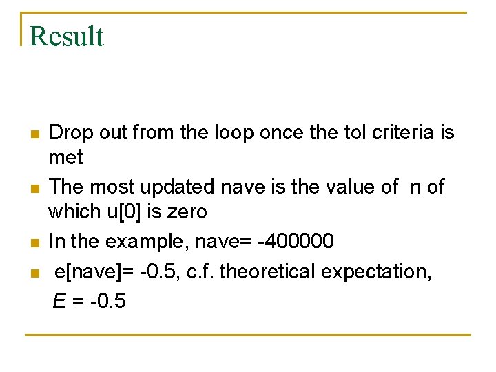
Result n n Drop out from the loop once the tol criteria is met The most updated nave is the value of n of which u[0] is zero In the example, nave= -400000 e[nave]= -0. 5, c. f. theoretical expectation, E = -0. 5

Profile of u(r) vs r

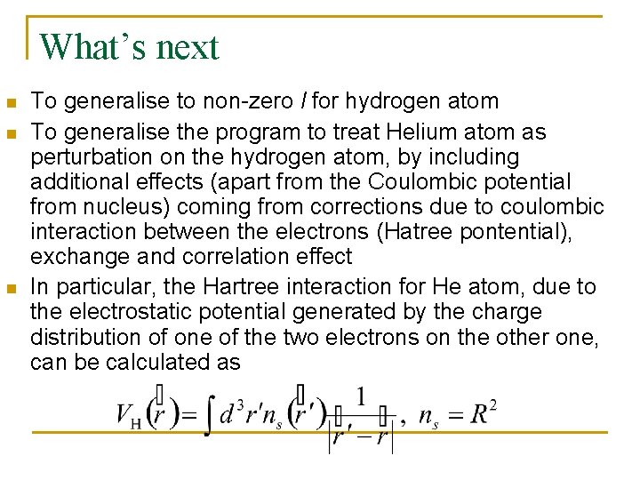
What’s next n n n To generalise to non-zero l for hydrogen atom To generalise the program to treat Helium atom as perturbation on the hydrogen atom, by including additional effects (apart from the Coulombic potential from nucleus) coming from corrections due to coulombic interaction between the electrons (Hatree pontential), exchange and correlation effect In particular, the Hartree interaction for He atom, due to the electrostatic potential generated by the charge distribution of one of the two electrons on the other one, can be calculated as

Hatree-Fock scheme n n The inclusion of Hatree interaction and exchange-correlation effect in He calculation has to be implemented in a self-consistent manner. The full program is called Hatree-Fock calculation, requiring extensive programming scheme that iterates the eigen energies of the multi-electron atom until the eigen-energies become convergent.

Conclusion n n The program developed in this talk calculates the eigen energy and the radial wave function of s-state hydrogen atom, and is readily expanded to treat cases of higher l In addition, the preliminary program presented here is the starting point to enter the full Hatree-Fock calculation for atoms with higher number of electrons The pdf version of the Mathematica code of this presentation can be found at the file “schrodinger 4. pdf”