VISUAL GEOMETRY GROUP Exploiting Duality Particularly the dual

VISUAL GEOMETRY GROUP Exploiting Duality (Particularly the dual of SVM) M. Pawan Kumar

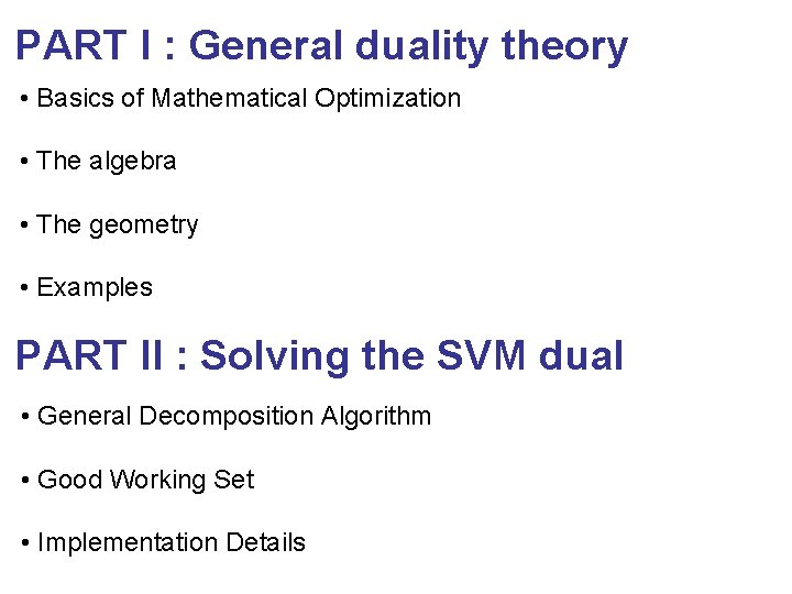
PART I : General duality theory • Basics of Mathematical Optimization • The algebra • The geometry • Examples PART II : Solving the SVM dual • General Decomposition Algorithm • Good Working Set • Implementation Details

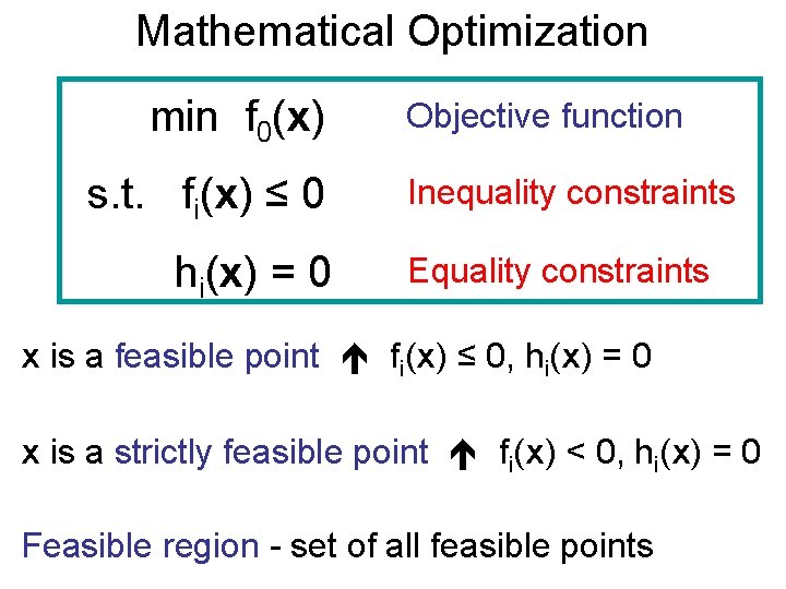
Mathematical Optimization min f 0(x) s. t. fi(x) ≤ 0 hi(x) = 0 Objective function Inequality constraints Equality constraints x is a feasible point fi(x) ≤ 0, hi(x) = 0 x is a strictly feasible point fi(x) < 0, hi(x) = 0 Feasible region - set of all feasible points

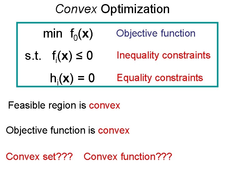
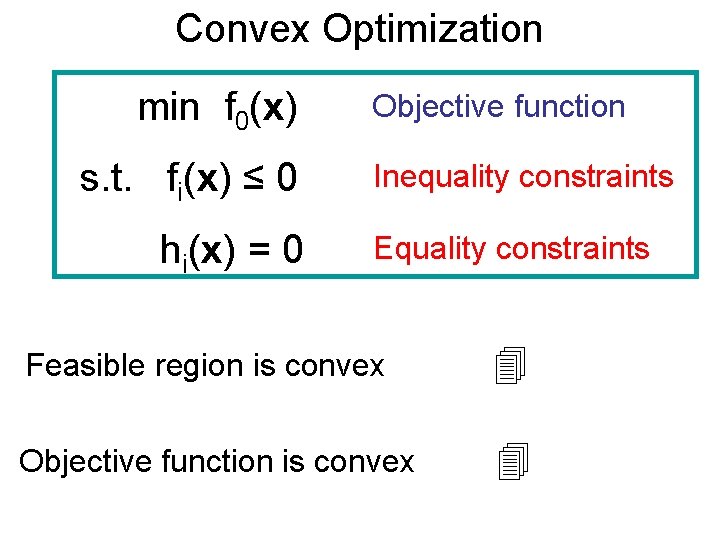
Convex Optimization min f 0(x) s. t. fi(x) ≤ 0 hi(x) = 0 Objective function Inequality constraints Equality constraints Feasible region is convex Objective function is convex Convex set? ? ? Convex function? ? ?

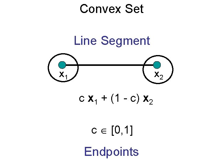
Convex Set Line Segment x 1 x 2 c x 1 + (1 - c) x 2 c [0, 1] Endpoints

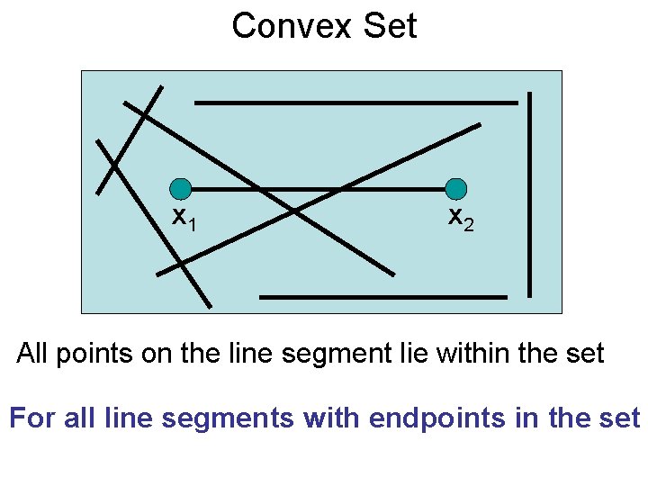
Convex Set x 1 x 2 All points on the line segment lie within the set For all line segments with endpoints in the set

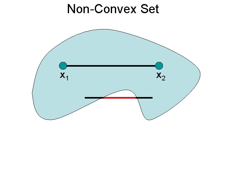
Non-Convex Set x 1 x 2

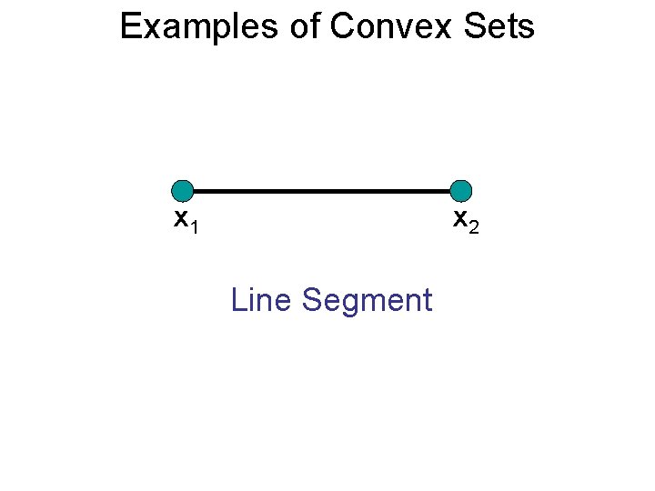
Examples of Convex Sets x 1 x 2 Line Segment

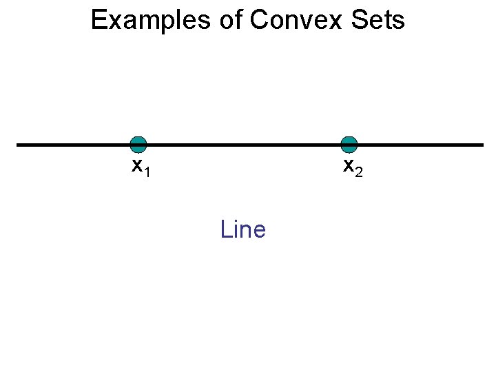
Examples of Convex Sets x 1 x 2 Line

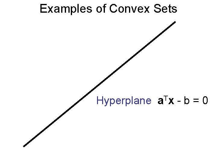
Examples of Convex Sets Hyperplane a. Tx - b = 0

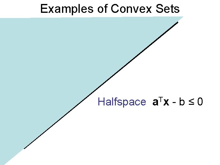
Examples of Convex Sets Halfspace a. Tx - b ≤ 0

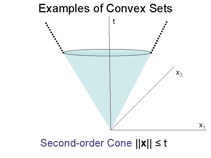
Examples of Convex Sets t x 2 x 1 Second-order Cone ||x|| ≤ t

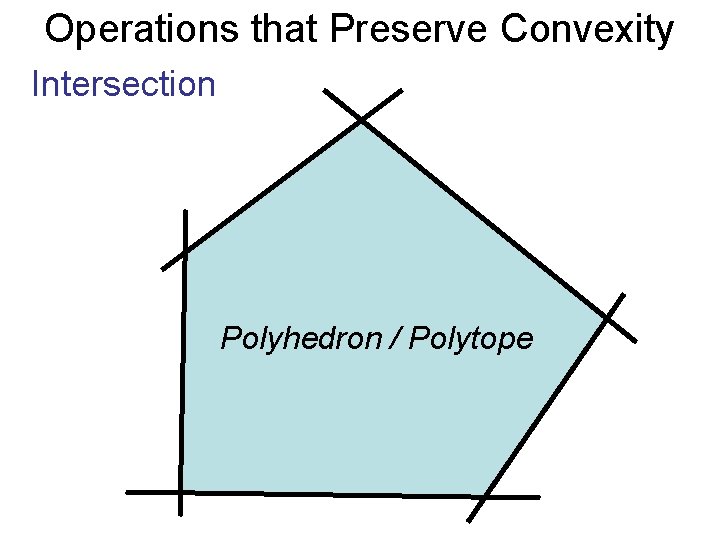
Operations that Preserve Convexity Intersection Polyhedron / Polytope

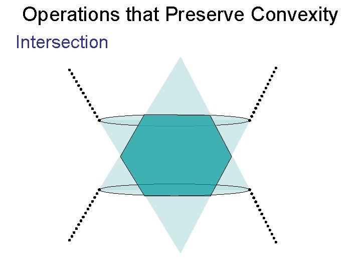
Operations that Preserve Convexity Intersection

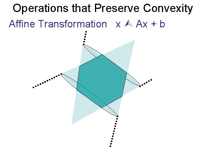
Operations that Preserve Convexity Affine Transformation x Ax + b

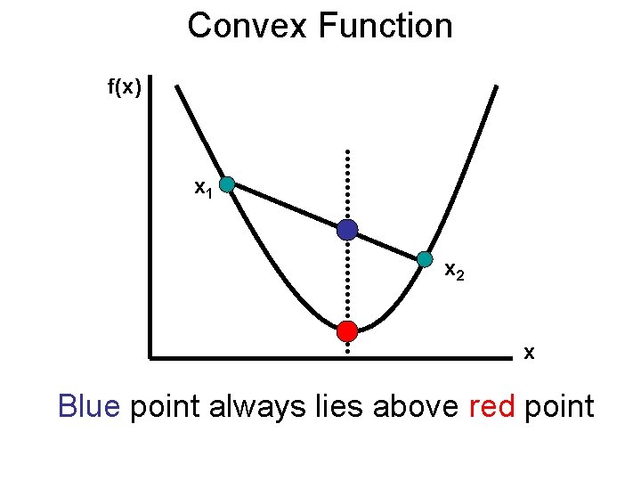
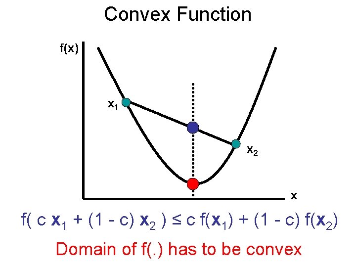
Convex Function f(x) x 1 x 2 x Blue point always lies above red point

Convex Function f(x) x 1 x 2 x f( c x 1 + (1 - c) x 2 ) ≤ c f(x 1) + (1 - c) f(x 2) Domain of f(. ) has to be convex

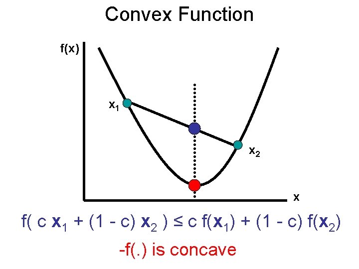
Convex Function f(x) x 1 x 2 x f( c x 1 + (1 - c) x 2 ) ≤ c f(x 1) + (1 - c) f(x 2) -f(. ) is concave

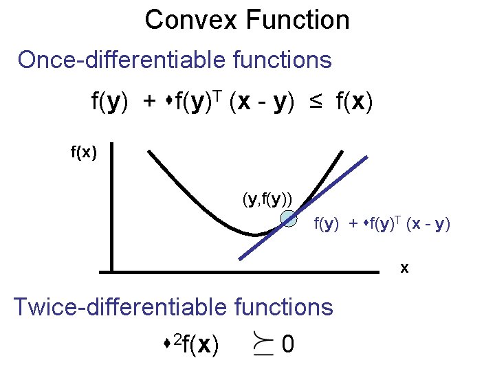
Convex Function Once-differentiable functions f(y) + f(y)T (x - y) ≤ f(x) (y, f(y)) f(y) + f(y)T (x - y) x Twice-differentiable functions 2 f(x) 0

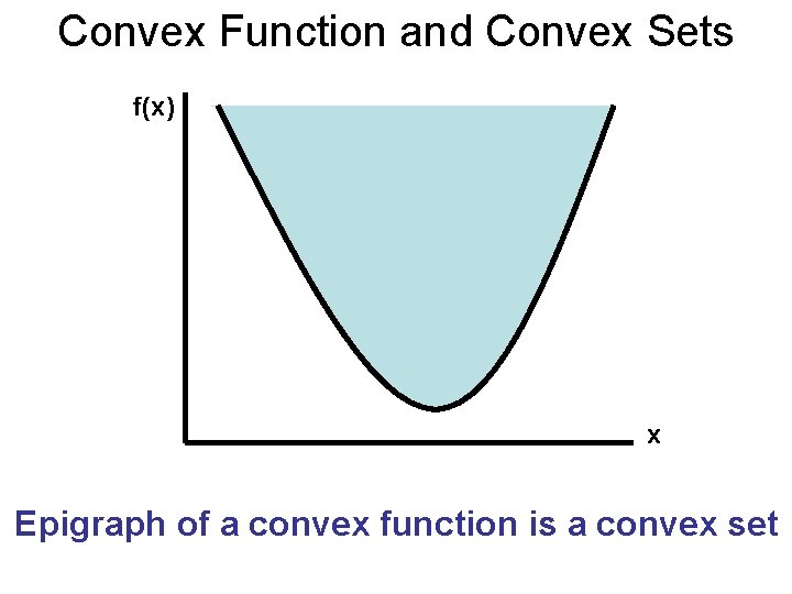
Convex Function and Convex Sets f(x) x Epigraph of a convex function is a convex set

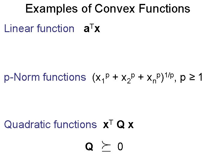
Examples of Convex Functions Linear function a. Tx p-Norm functions (x 1 p + x 2 p + xnp)1/p, p ≥ 1 Quadratic functions x. T Q x Q 0

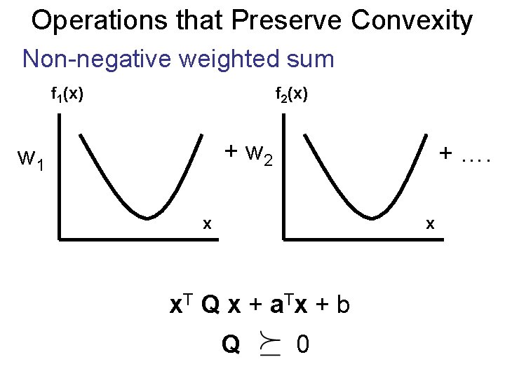
Operations that Preserve Convexity Non-negative weighted sum f 1(x) f 2(x) + w 2 w 1 + …. x x x. T Q x + a. T x + b Q 0

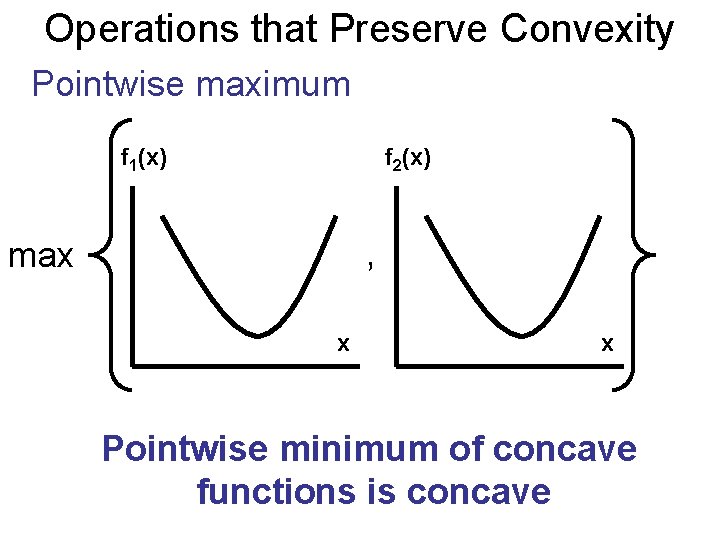
Operations that Preserve Convexity Pointwise maximum f 1(x) f 2(x) , max x x Pointwise minimum of concave functions is concave

Convex Optimization min f 0(x) s. t. fi(x) ≤ 0 hi(x) = 0 Objective function Inequality constraints Equality constraints Feasible region is convex Objective function is convex

PART I : General duality theory • Basics of Mathematical Optimization • The algebra • The geometry • Examples PART II : Solving the SVM dual • General Decomposition Algorithm • Good Working Set • Implementation Details

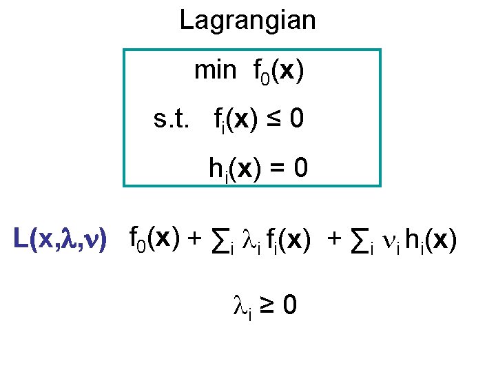
Lagrangian min f 0(x) s. t. fi(x) ≤ 0 hi(x) = 0 L(x, , ) f 0(x) + ∑i i fi(x) + ∑i i hi(x) i ≥ 0

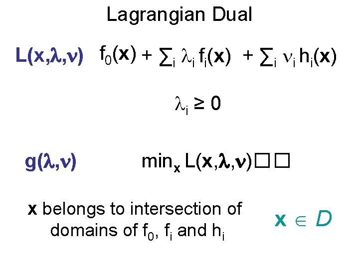
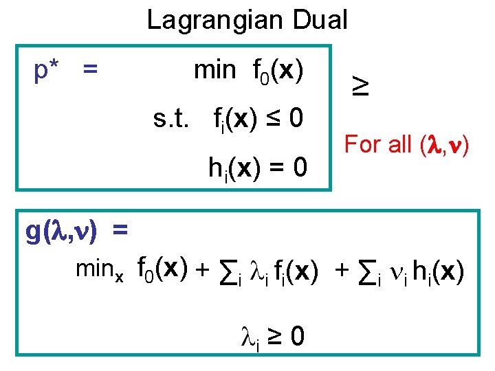
Lagrangian Dual L(x, , ) f 0(x) + ∑i i fi(x) + ∑i i hi(x) i ≥ 0 g( , ) minx L(x, , )�� x belongs to intersection of domains of f 0, fi and hi x D

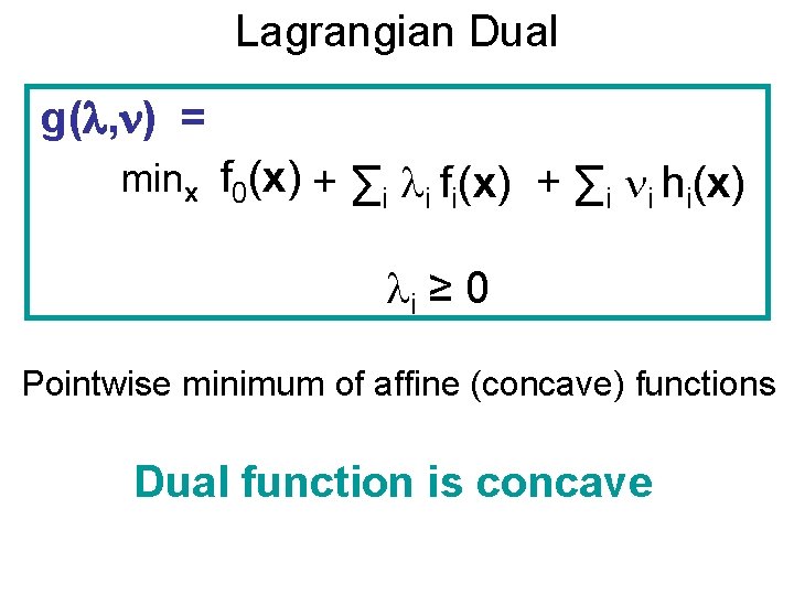
Lagrangian Dual g( , ) = minx f 0(x) + ∑i i fi(x) + ∑i i hi(x) i ≥ 0 Pointwise minimum of affine (concave) functions Dual function is concave

Lagrangian Dual p* = min f 0(x) s. t. fi(x) ≤ 0 hi(x) = 0 ≥ For all ( , ) g( , ) = minx f 0(x) + ∑i i fi(x) + ∑i i hi(x) i ≥ 0

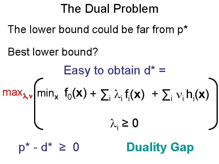
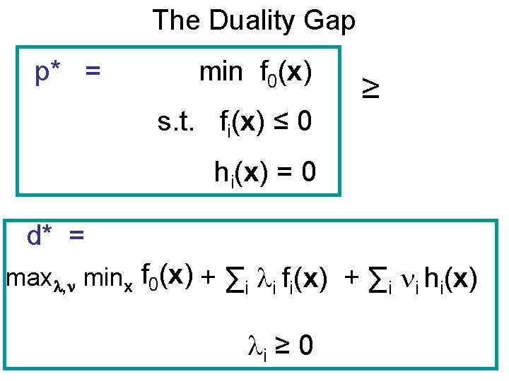
The Dual Problem The lower bound could be far from p* Best lower bound? Easy to obtain d* = max , minx f 0(x) + ∑ f (x) + ∑ h (x) i i i i ≥ 0 p* - d* ≥ 0 Duality Gap

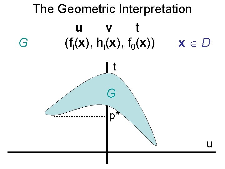
The Geometric Interpretation u v t (fi(x), hi(x), f 0(x)) G x D t G p* u

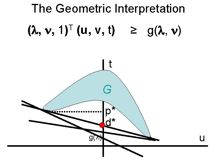
The Geometric Interpretation ( , , 1)T (u, v, t) ≥ g( , ) t G p* d* g( ) u

The Duality Gap p* = min f 0(x) s. t. fi(x) ≤ 0 ≥ hi(x) = 0 d* = max , minx f 0(x) + ∑i i fi(x) + ∑i i hi(x) i ≥ 0

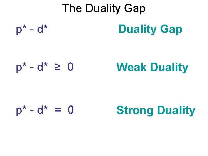
The Duality Gap p* - d* ≥ 0 Weak Duality p* - d* = 0 Strong Duality

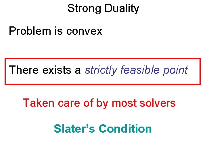
Strong Duality Problem is convex There exists a strictly feasible point Taken care of by most solvers Slater’s Condition

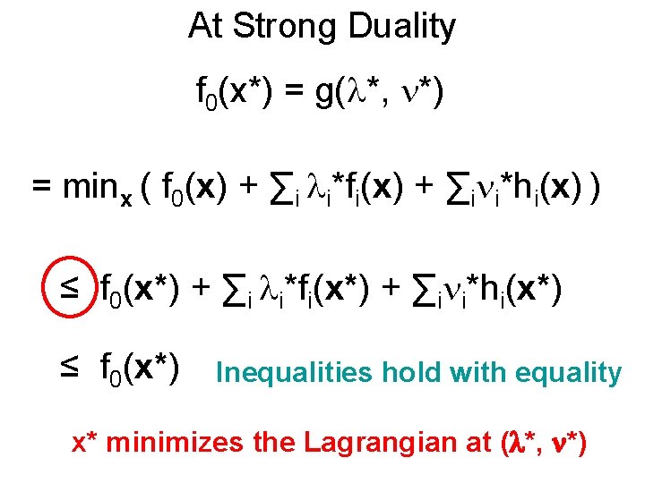
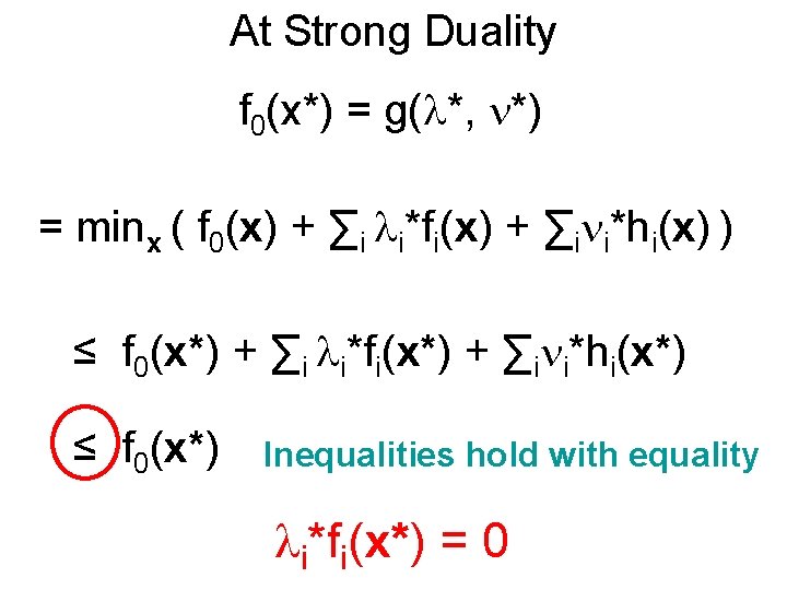
At Strong Duality f 0(x*) = g( *, *) = minx ( f 0(x) + ∑i i*fi(x) + ∑i i*hi(x) ) ≤ f 0(x*) + ∑i i*fi(x*) + ∑i i*hi(x*) ≤ f 0(x*) Inequalities hold with equality x* minimizes the Lagrangian at ( *, *)

At Strong Duality f 0(x*) = g( *, *) = minx ( f 0(x) + ∑i i*fi(x) + ∑i i*hi(x) ) ≤ f 0(x*) + ∑i i*fi(x*) + ∑i i*hi(x*) ≤ f 0(x*) Inequalities hold with equality i*fi(x*) = 0

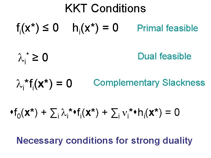
KKT Conditions fi(x*) ≤ 0 hi(x*) = 0 i* ≥ 0 i*fi(x*) = 0 Primal feasible Dual feasible Complementary Slackness f 0(x*) + ∑i i* fi(x*) + ∑i i* hi(x*) = 0 Necessary conditions for strong duality

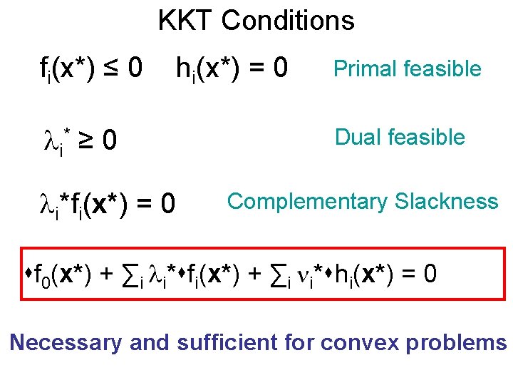
KKT Conditions fi(x*) ≤ 0 hi(x*) = 0 i* ≥ 0 i*fi(x*) = 0 Primal feasible Dual feasible Complementary Slackness f 0(x*) + ∑i i* fi(x*) + ∑i i* hi(x*) = 0 Necessary and sufficient for convex problems

PART I : General duality theory • Basics of Mathematical Optimization • The algebra • The geometry • Examples PART II : Solving the SVM dual • General Decomposition Algorithm • Good Working Set • Implementation Details

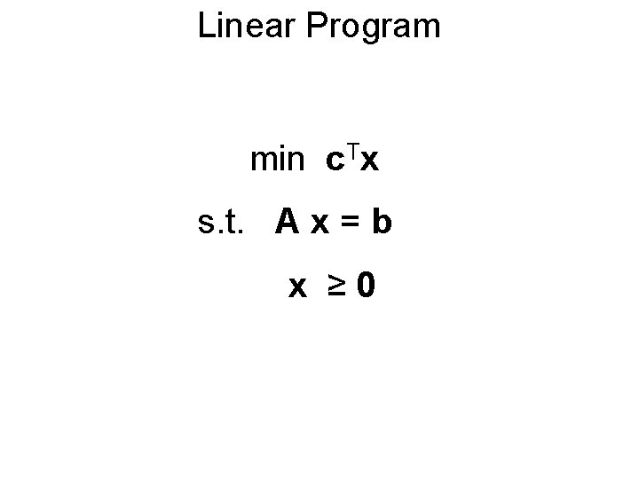
Linear Program min c. Tx s. t. A x = b x ≥ 0

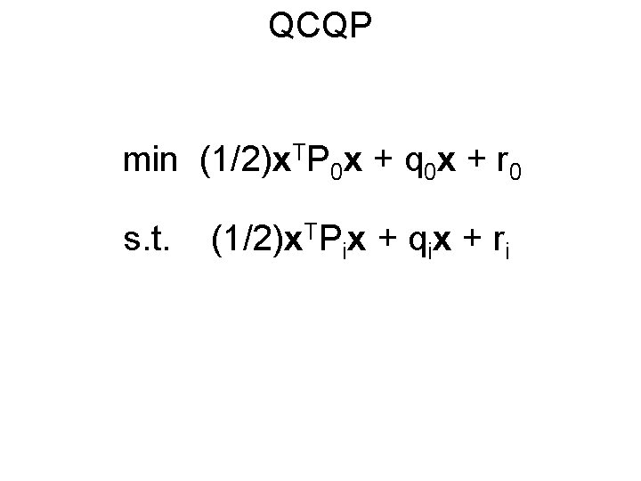
QCQP min (1/2)x. TP 0 x + q 0 x + r 0 s. t. (1/2)x. TPix + qix + ri

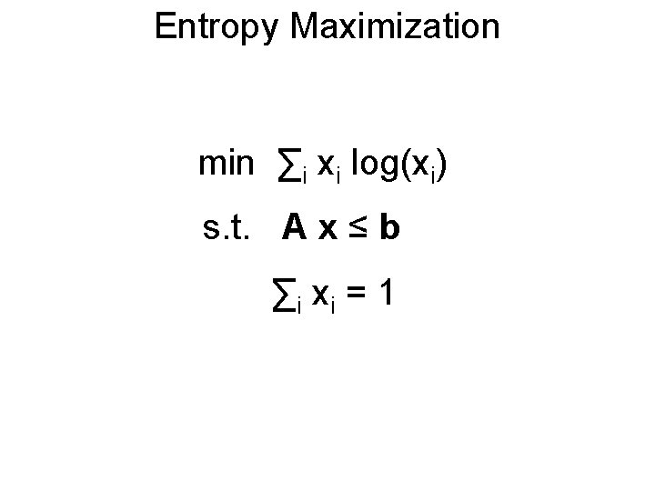
Entropy Maximization min ∑i xi log(xi) s. t. A x ≤ b ∑i xi = 1

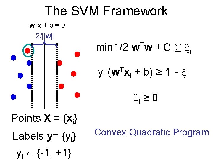
The SVM Framework w Tx + b = 0 2/||w|| min 1/2 w. Tw + C i yi (w. Txi + b) ≥ 1 - i i ≥ 0 Points X = {xi} Labels y= {yi} yi {-1, +1} Convex Quadratic Program

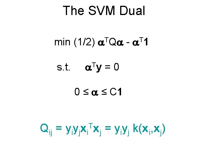
The SVM Dual min (1/2) TQ - T 1 s. t. Ty = 0 0 ≤ ≤ C 1 Qij = yiyjxi. Txj = yiyj k(xi, xj)

PART I : General duality theory • Basics of Mathematical Optimization • The algebra • The geometry • Examples PART II : Solving the SVM dual • General Decomposition Algorithm • Good Working Set • Implementation Details

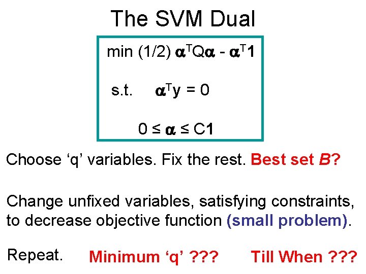
The SVM Dual min (1/2) TQ - T 1 s. t. Ty = 0 0 ≤ ≤ C 1 Choose ‘q’ variables. Fix the rest. Best set B? Change unfixed variables, satisfying constraints, to decrease objective function (small problem). Repeat. Minimum ‘q’ ? ? ? Till When ? ? ?

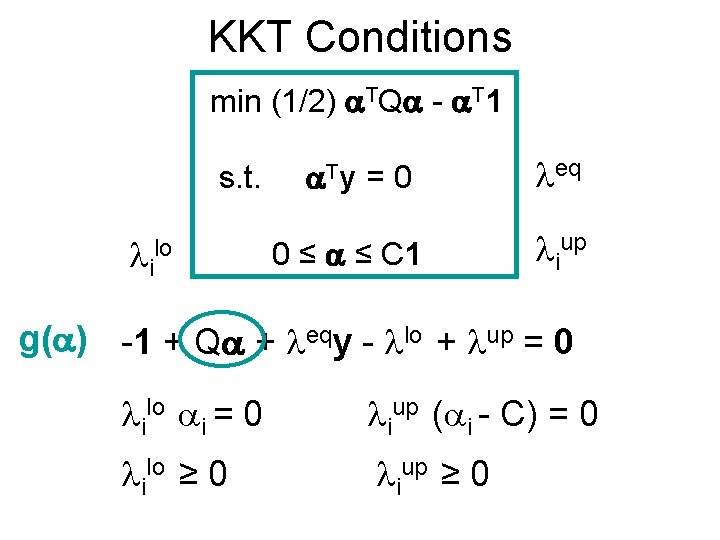
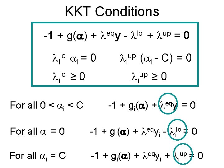
KKT Conditions min (1/2) TQ - T 1 s. t. ilo Ty =0 0 ≤ ≤ C 1 eq iup g( ) -1 + Q + eqy - lo + up = 0 ilo i = 0 iup ( i - C) = 0 ilo ≥ 0 iup ≥ 0

KKT Conditions -1 + g( ) + eqy - lo + up = 0 ilo i = 0 ilo ≥ 0 For all 0 < i < C iup ( i - C) = 0 iup ≥ 0 -1 + gi( ) + eqyi = 0 For all i = 0 -1 + gi( ) + eqyi - ilo = 0 For all i = C -1 + gi( ) + eqyi + iup = 0

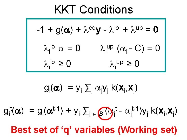
KKT Conditions -1 + g( ) + eqy - lo + up = 0 ilo i = 0 ilo ≥ 0 iup ( i - C) = 0 iup ≥ 0 gi( ) = yi ∑j jyj k(xi, xj) git( ) = gi( t-1) + yi ∑j B ( jt - jt-1)yj k(xi, xj) Best set of ‘q’ variables (Working set)

PART I : General duality theory • Basics of Mathematical Optimization • The algebra • The geometry • Examples PART II : Solving the SVM dual • General Decomposition Algorithm • Good Working Set • Implementation Details

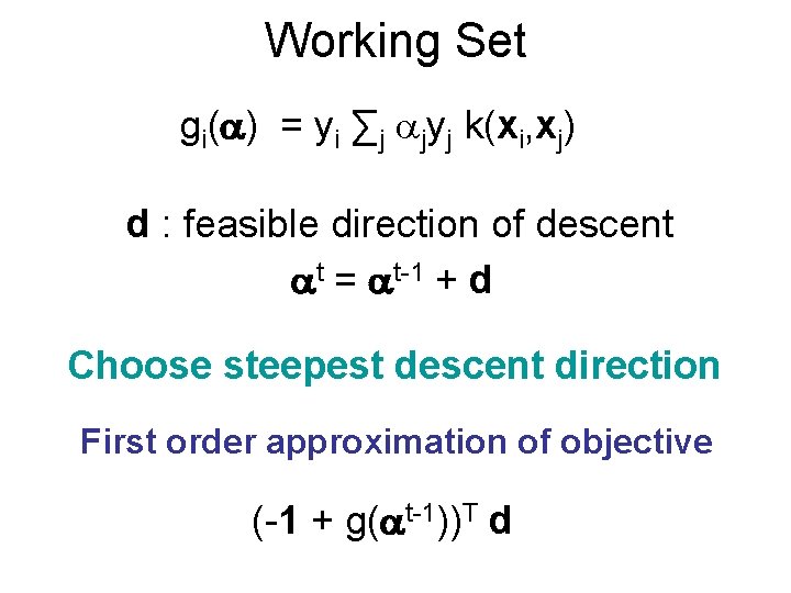
Working Set gi( ) = yi ∑j jyj k(xi, xj) d : feasible direction of descent t = t-1 + d Choose steepest descent direction First order approximation of objective (-1 + g( t-1))T d

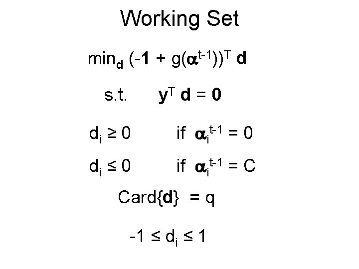
Working Set mind (-1 + g( t-1))T d s. t. y. T d = 0 di ≥ 0 if it-1 = 0 di ≤ 0 if it-1 = C Card{d} = q -1 ≤ di ≤ 1

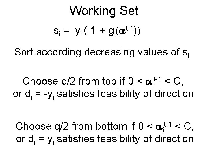
Working Set si = yi (-1 + gi( t-1)) Sort according decreasing values of si Choose q/2 from top if 0 < it-1 < C, or di = -yi satisfies feasibility of direction Choose q/2 from bottom if 0 < it-1 < C, or di = yi satisfies feasibility of direction

Working Set mind (-1 + g( t-1))T d s. t. y. T d = 0 di ≥ 0 if it-1 = 0 di ≤ 0 if it-1 = C Card{d} = q -1 ≤ di ≤ 1

PART I : General duality theory • Basics of Mathematical Optimization • The algebra • The geometry • Examples PART II : Solving the SVM dual • General Decomposition Algorithm • Good Working Set • Implementation Details

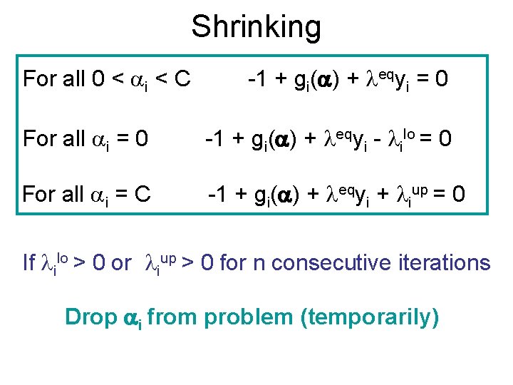
Shrinking For all 0 < i < C -1 + gi( ) + eqyi = 0 For all i = 0 -1 + gi( ) + eqyi - ilo = 0 For all i = C -1 + gi( ) + eqyi + iup = 0 If ilo > 0 or iup > 0 for n consecutive iterations Drop i from problem (temporarily)

Caching Kernel evaluation can be expensive Cache them in a least-recently-used manner Choose q’ variables where cache available

Results Those who have used SVMlight : You know that it works very well. Those who haven’t used SVMlight : It works very well. See paper. Download.

Questions? ? ?