Topic 16 Multicollinearity and Polynomial Regression Outline Multicollinearity

Topic 16: Multicollinearity and Polynomial Regression

Outline • Multicollinearity • Polynomial regression

An example (KNNL p 256) • The P-value for ANOVA F-test is <. 0001 • The P values for the individual regression coefficients are 0. 1699, 0. 2849, and 0. 1896 • None of these are near our standard significance level of 0. 05 • What is the explanation? Multicollinearity!!!

Multicollinearity • Numerical analysis problem in that the matrix X΄X is close to singular and is therefore difficult to invert accurately • Statistical problem in that there is too much correlation among the explanatory variables and it is therefore difficult to determine the regression coefficients

Multicollinearity • Solve the statistical problem and the numerical problem will also be solved – We want to refine a model that currently has redundancy in the explanatory variables – Do this regardless if X΄X can be inverted without difficulty

Multicollinearity • Extreme cases can help us understand the problems caused by multicollinearity – Assume columns in X matrix were uncorrelated • Type I and Type II SS will be the same • The contribution of each explanatory variable to the model is the same whether or not the other explanatory variables are in the model

Multicollinearity – Suppose a linear combination of the explanatory variables is a constant • Example: X 1 = X 2 → X 1 -X 2 = 0 • Example: 3 X 1 -X 2 = 5 • Example: SAT total = SATV + SATM • The Type II SS for the X’s involved will all be zero

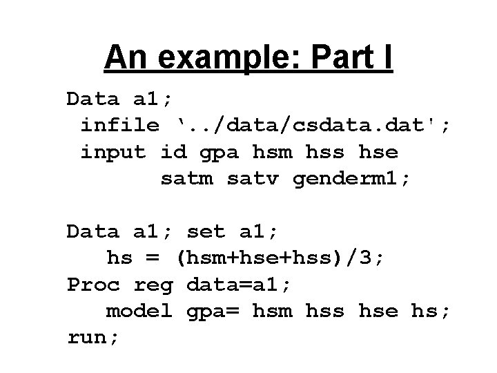
An example: Part I Data a 1; infile ‘. . /data/csdata. dat'; input id gpa hsm hss hse satm satv genderm 1; Data a 1; set a 1; hs = (hsm+hse+hss)/3; Proc reg data=a 1; model gpa= hsm hss hse hs; run;

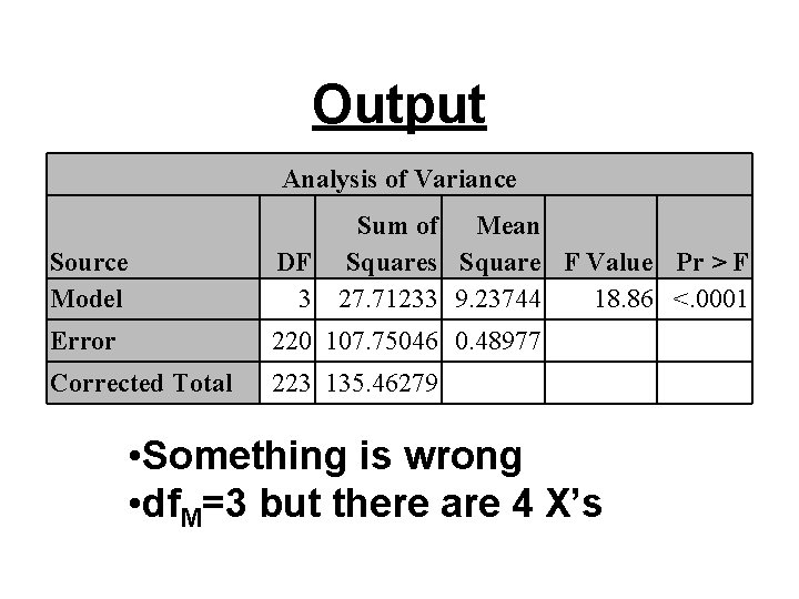
Output Analysis of Variance Source Model Sum of Mean DF Squares Square F Value Pr > F 3 27. 71233 9. 23744 18. 86 <. 0001 Error 220 107. 75046 0. 48977 Corrected Total 223 135. 46279 • Something is wrong • df. M=3 but there are 4 X’s

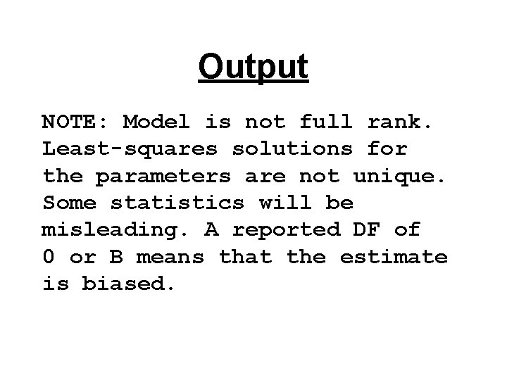
Output NOTE: Model is not full rank. Least-squares solutions for the parameters are not unique. Some statistics will be misleading. A reported DF of 0 or B means that the estimate is biased.

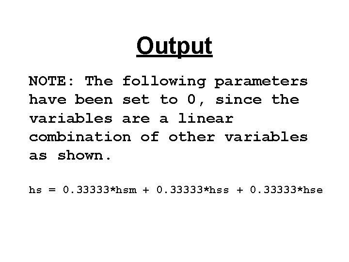
Output NOTE: The following parameters have been set to 0, since the variables are a linear combination of other variables as shown. hs = 0. 33333*hsm + 0. 33333*hss + 0. 33333*hse

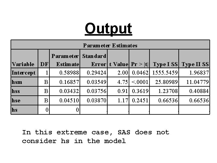
Output Parameter Estimates Parameter Standard Variable DF Estimate Error t Value Pr > |t| Type I SS Type II SS Intercept 1 0. 58988 0. 29424 2. 00 0. 0462 1555. 5459 1. 96837 hsm B 0. 16857 0. 03549 4. 75 <. 0001 25. 80989 11. 04779 hss B 0. 03432 0. 03756 0. 91 0. 3619 1. 23708 0. 40884 hse B 0. 04510 0. 03870 1. 17 0. 2451 0. 66536 hs 0 0 . . . In this extreme case, SAS does not consider hs in the model

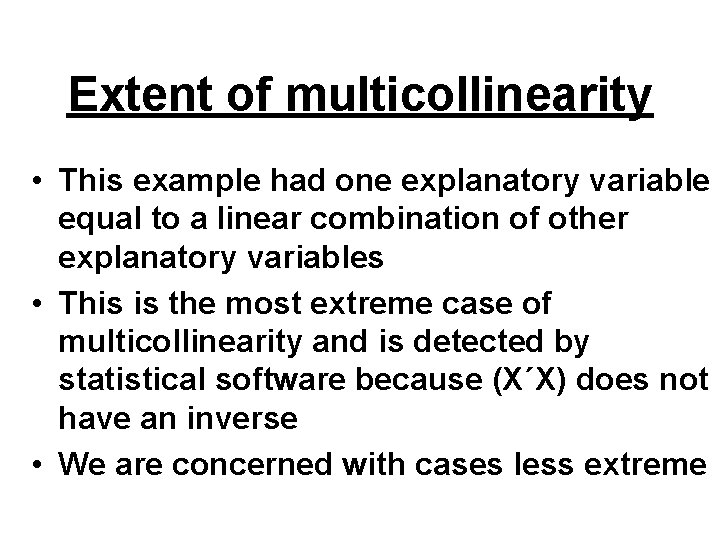
Extent of multicollinearity • This example had one explanatory variable equal to a linear combination of other explanatory variables • This is the most extreme case of multicollinearity and is detected by statistical software because (X΄X) does not have an inverse • We are concerned with cases less extreme

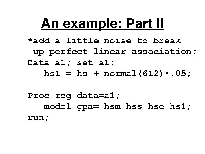
An example: Part II *add a little noise to break up perfect linear association; Data a 1; set a 1; hs 1 = hs + normal(612)*. 05; Proc reg data=a 1; model gpa= hsm hss hse hs 1; run;

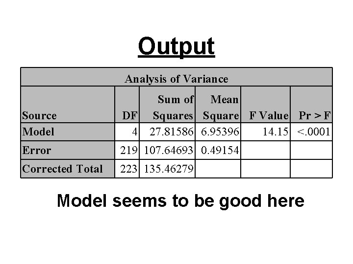
Output Analysis of Variance Source Model Sum of Mean DF Squares Square F Value Pr > F 4 27. 81586 6. 95396 14. 15 <. 0001 Error 219 107. 64693 0. 49154 Corrected Total 223 135. 46279 Model seems to be good here

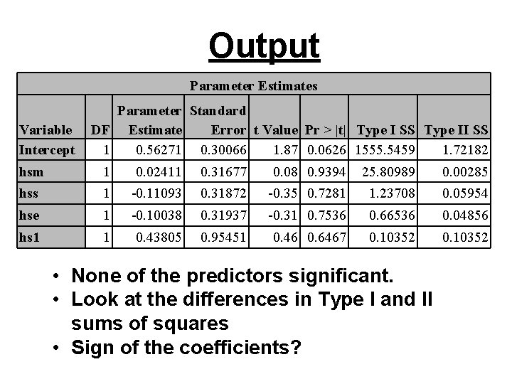
Output Parameter Estimates Variable Intercept Parameter Standard DF Estimate Error t Value Pr > |t| Type I SS Type II SS 1 0. 56271 0. 30066 1. 87 0. 0626 1555. 5459 1. 72182 hsm 1 0. 02411 0. 31677 0. 08 0. 9394 25. 80989 0. 00285 hss 1 -0. 11093 0. 31872 -0. 35 0. 7281 1. 23708 0. 05954 hse 1 -0. 10038 0. 31937 -0. 31 0. 7536 0. 66536 0. 04856 hs 1 1 0. 43805 0. 95451 0. 46 0. 6467 0. 10352 • None of the predictors significant. • Look at the differences in Type I and II sums of squares • Sign of the coefficients?

Effects of multicollinearity • Regression coefficients are not well estimated and may be meaningless • Similarly for standard errors of these estimates • Type I SS and Type II SS will differ • R 2 and predicted values are usually ok

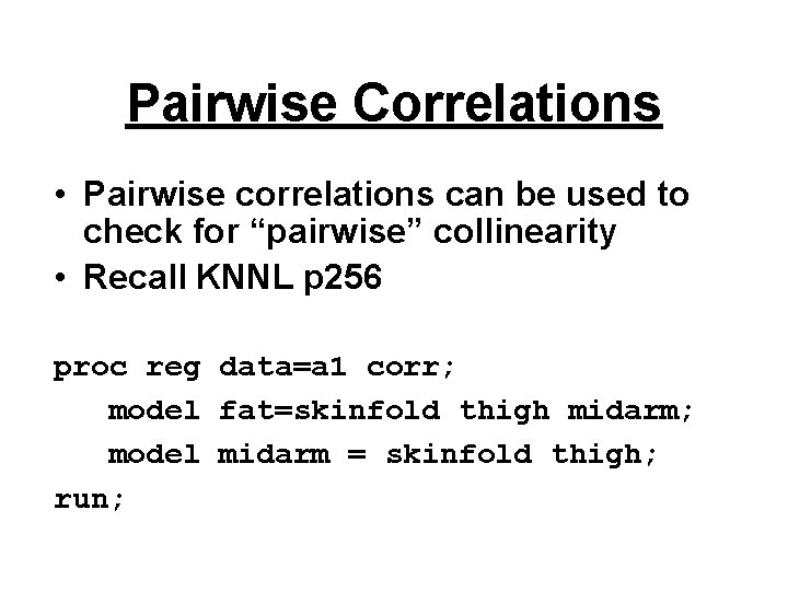
Pairwise Correlations • Pairwise correlations can be used to check for “pairwise” collinearity • Recall KNNL p 256 proc reg data=a 1 corr; model fat=skinfold thigh midarm; model midarm = skinfold thigh; run;

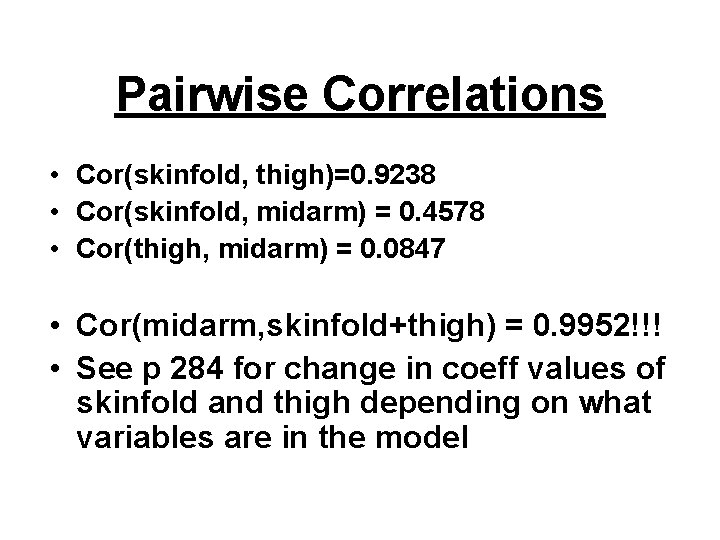
Pairwise Correlations • Cor(skinfold, thigh)=0. 9238 • Cor(skinfold, midarm) = 0. 4578 • Cor(thigh, midarm) = 0. 0847 • Cor(midarm, skinfold+thigh) = 0. 9952!!! • See p 284 for change in coeff values of skinfold and thigh depending on what variables are in the model

Polynomial regression • We can fit a quadratic, cubic, etc. relationship by defining squares, cubes, etc. , of a single X in a data step and using them as additional explanatory variables • We can do this with more than one explanatory variable if needed • Issue: When we do this we generally create a multicollinearity problem

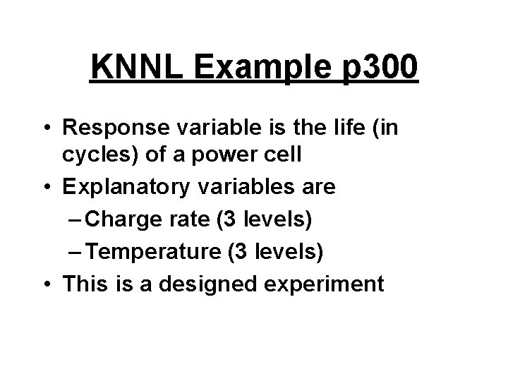
KNNL Example p 300 • Response variable is the life (in cycles) of a power cell • Explanatory variables are – Charge rate (3 levels) – Temperature (3 levels) • This is a designed experiment

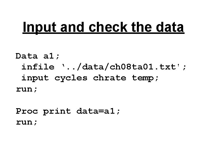
Input and check the data Data a 1; infile ‘. . /data/ch 08 ta 01. txt'; input cycles chrate temp; run; Proc print data=a 1; run;

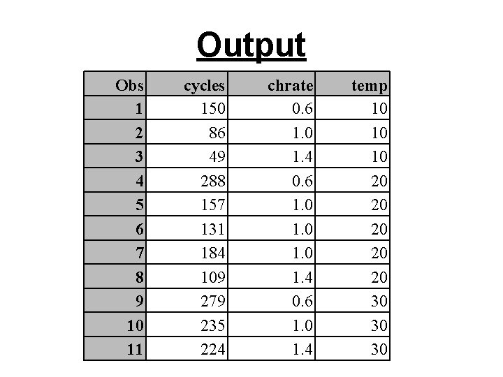
Output Obs 1 2 3 4 5 6 7 8 9 10 11 cycles 150 86 49 288 157 131 184 109 279 235 224 chrate 0. 6 1. 0 1. 4 temp 10 10 10 20 20 20 30 30 30

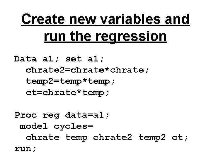
Create new variables and run the regression Data a 1; set a 1; chrate 2=chrate*chrate; temp 2=temp*temp; ct=chrate*temp; Proc reg data=a 1; model cycles= chrate temp chrate 2 temp 2 ct; run;

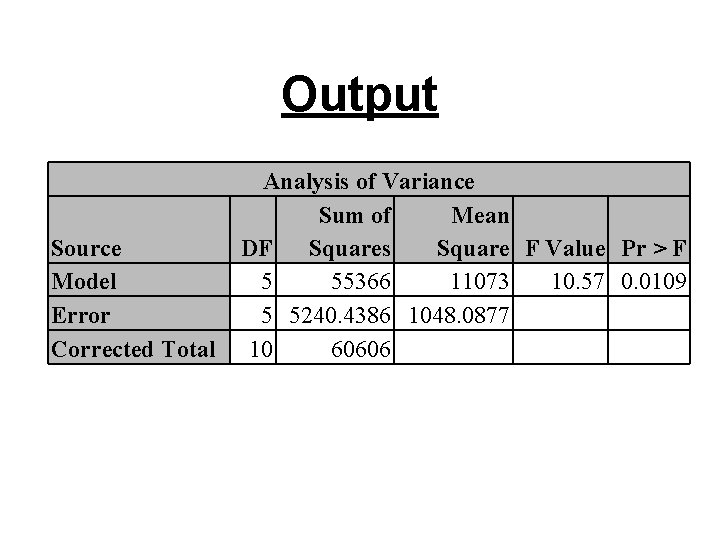
Output Source Model Error Corrected Total Analysis of Variance Sum of Mean DF Squares Square F Value Pr > F 5 55366 11073 10. 57 0. 0109 5 5240. 4386 1048. 0877 10 60606

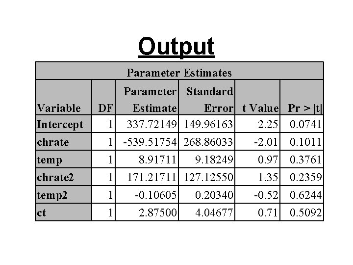
Output Parameter Estimates Variable Intercept chrate temp chrate 2 temp 2 ct DF 1 1 1 Parameter Estimate 337. 72149 -539. 51754 8. 91711 171. 21711 -0. 10605 2. 87500 Standard Error t Value Pr > |t| 149. 96163 2. 25 0. 0741 268. 86033 -2. 01 0. 1011 9. 18249 0. 97 0. 3761 127. 12550 1. 35 0. 2359 0. 20340 -0. 52 0. 6244 4. 04677 0. 71 0. 5092

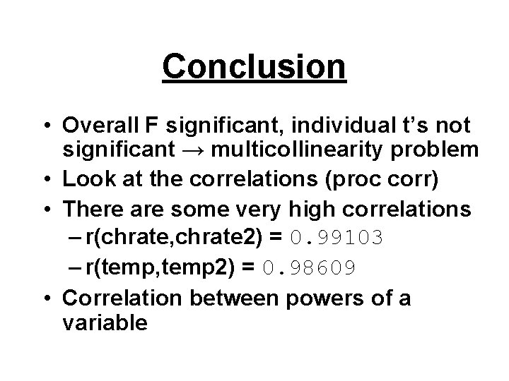
Conclusion • Overall F significant, individual t’s not significant → multicollinearity problem • Look at the correlations (proc corr) • There are some very high correlations – r(chrate, chrate 2) = 0. 99103 – r(temp, temp 2) = 0. 98609 • Correlation between powers of a variable

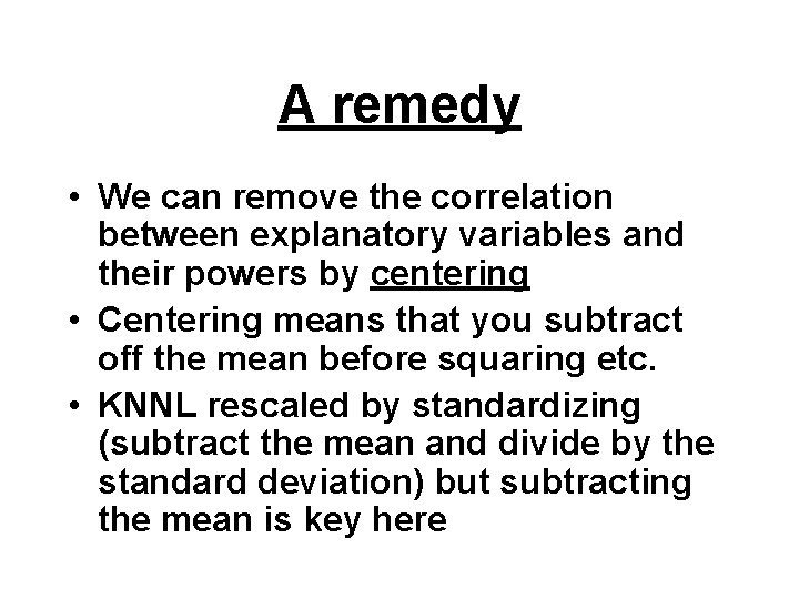
A remedy • We can remove the correlation between explanatory variables and their powers by centering • Centering means that you subtract off the mean before squaring etc. • KNNL rescaled by standardizing (subtract the mean and divide by the standard deviation) but subtracting the mean is key here

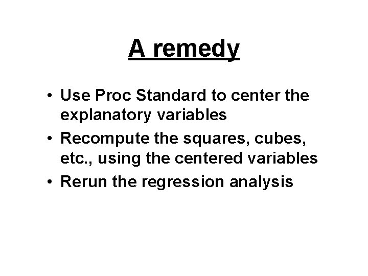
A remedy • Use Proc Standard to center the explanatory variables • Recompute the squares, cubes, etc. , using the centered variables • Rerun the regression analysis

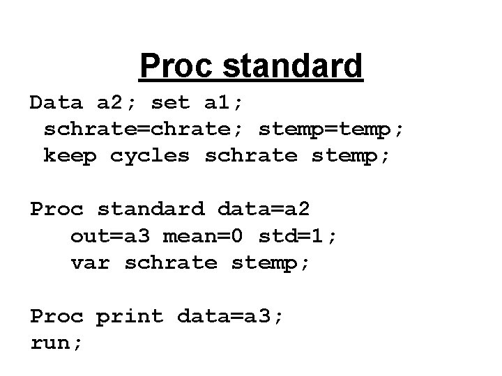
Proc standard Data a 2; set a 1; schrate=chrate; stemp=temp; keep cycles schrate stemp; Proc standard data=a 2 out=a 3 mean=0 std=1; var schrate stemp; Proc print data=a 3; run;

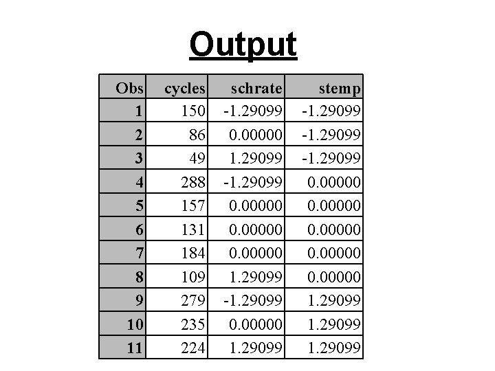
Output Obs 1 2 3 4 5 6 7 8 9 10 11 cycles 150 86 49 288 157 131 184 109 279 235 224 schrate -1. 29099 0. 00000 1. 29099 -1. 29099 0. 00000 1. 29099 stemp -1. 29099 0. 00000 1. 29099

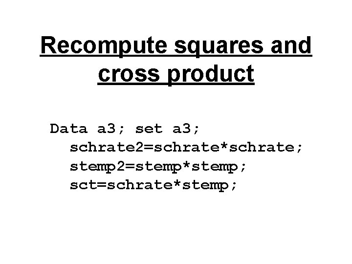
Recompute squares and cross product Data a 3; set a 3; schrate 2=schrate*schrate; stemp 2=stemp*stemp; sct=schrate*stemp;

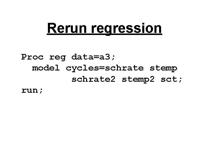
Rerun regression Proc reg data=a 3; model cycles=schrate stemp schrate 2 stemp 2 sct; run;

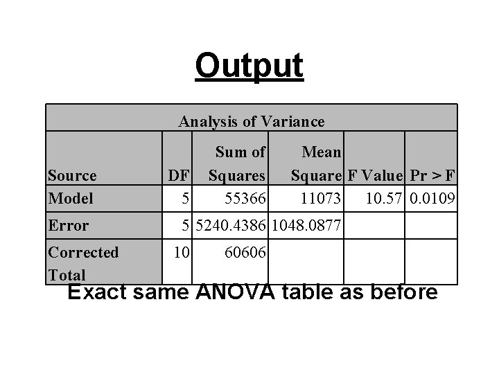
Output Analysis of Variance Source Model Error Corrected Total DF 5 Sum of Squares 55366 Mean Square F Value Pr > F 11073 10. 57 0. 0109 5 5240. 4386 1048. 0877 10 60606 Exact same ANOVA table as before

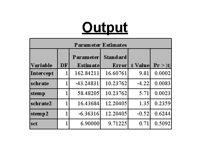
Output Parameter Estimates Variable Intercept Parameter Standard DF Estimate Error t Value Pr > |t| 1 162. 84211 16. 60761 9. 81 0. 0002 schrate 1 -43. 24831 10. 23762 -4. 22 0. 0083 stemp 1 58. 48205 10. 23762 5. 71 0. 0023 schrate 2 1 16. 43684 12. 20405 1. 35 0. 2359 stemp 2 1 -6. 36316 12. 20405 -0. 52 0. 6244 sct 1 6. 90000 9. 71225 0. 71 0. 5092

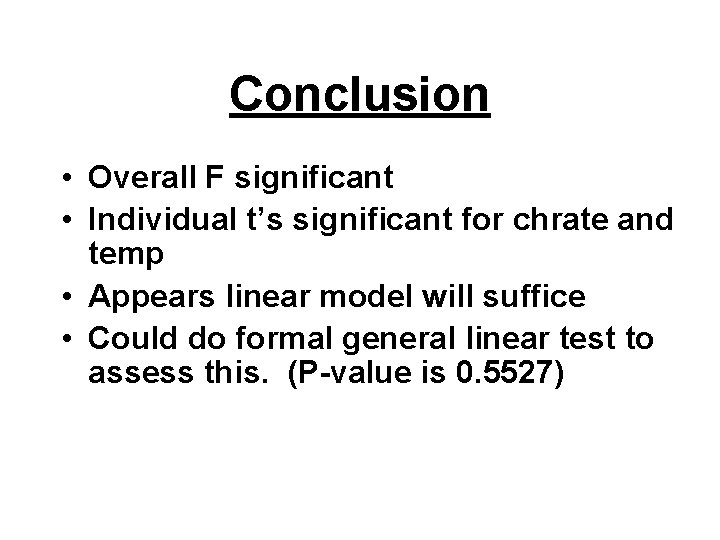
Conclusion • Overall F significant • Individual t’s significant for chrate and temp • Appears linear model will suffice • Could do formal general linear test to assess this. (P-value is 0. 5527)

Last slide • We went over KNNL 7. 6 and 8. 1. • We used programs Topic 16. sas to generate the output for today