Chapter 13 Nonlinear and Multiple Regression 13 1

Chapter 13 Nonlinear and Multiple Regression

13. 1 Aptness of the Model and Model Checking

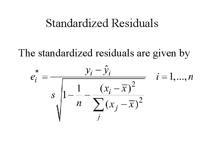
Standardized Residuals The standardized residuals are given by

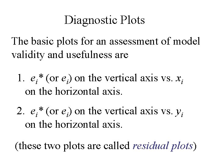
Diagnostic Plots The basic plots for an assessment of model validity and usefulness are 1. ei* (or ei) on the vertical axis vs. xi on the horizontal axis. 2. ei* (or ei) on the vertical axis vs. yi on the horizontal axis. (these two plots are called residual plots)

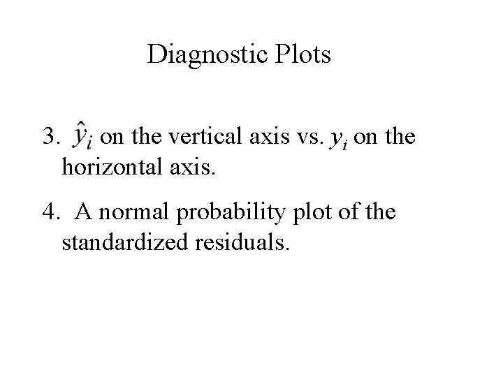
Diagnostic Plots 3. on the vertical axis vs. yi on the horizontal axis. 4. A normal probability plot of the standardized residuals.

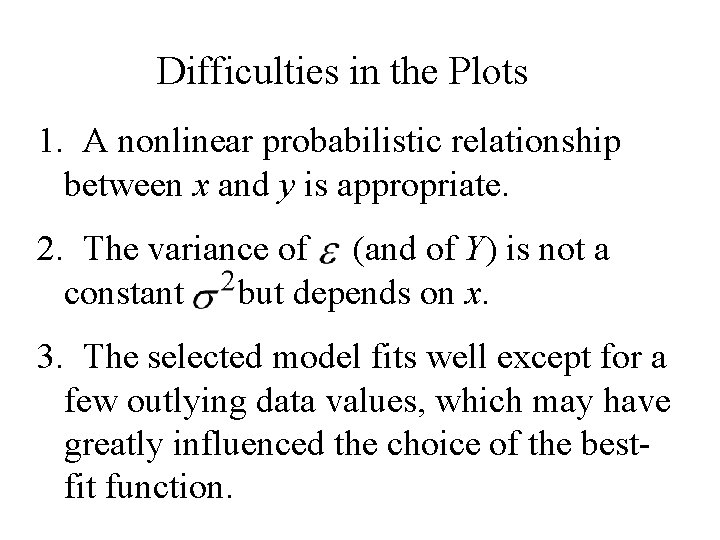
Difficulties in the Plots 1. A nonlinear probabilistic relationship between x and y is appropriate. 2. The variance of (and of Y) is not a constant but depends on x. 3. The selected model fits well except for a few outlying data values, which may have greatly influenced the choice of the bestfit function.

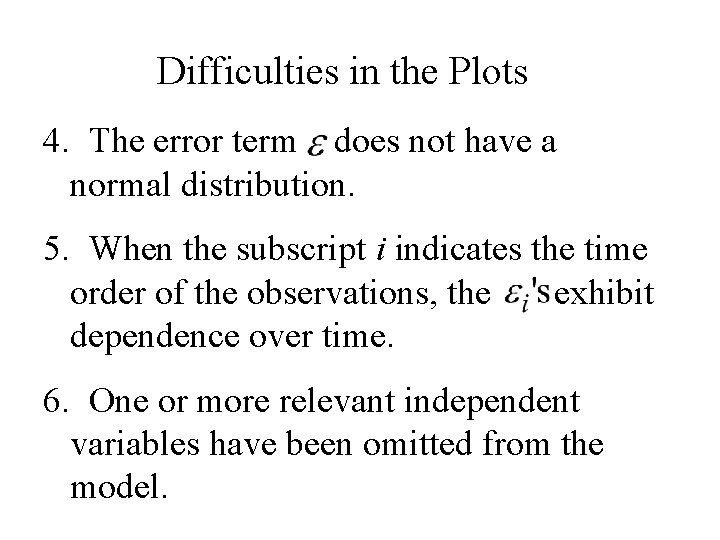
Difficulties in the Plots 4. The error term does not have a normal distribution. 5. When the subscript i indicates the time order of the observations, the exhibit dependence over time. 6. One or more relevant independent variables have been omitted from the model.

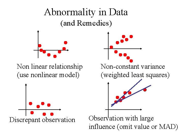
Abnormality in Data (and Remedies) Non linear relationship (use nonlinear model) Discrepant observation Non-constant variance (weighted least squares) Observation with large influence (omit value or MAD)

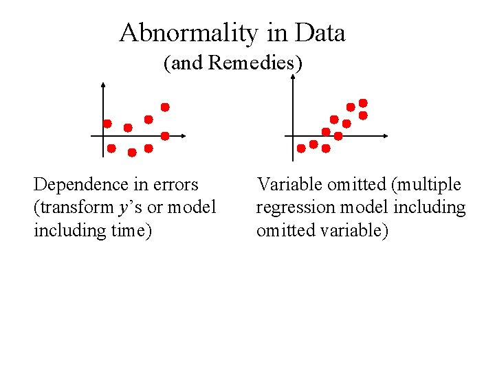
Abnormality in Data (and Remedies) Dependence in errors (transform y’s or model including time) Variable omitted (multiple regression model including omitted variable)

13. 2 Regression With Transformed Variables

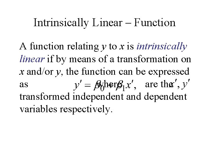
Intrinsically Linear – Function A function relating y to x is intrinsically linear if by means of a transformation on x and/or y, the function can be expressed as where are the transformed independent and dependent variables respectively.

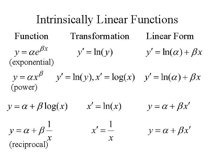
Intrinsically Linear Functions Function (exponential) (power) (reciprocal) Transformation Linear Form

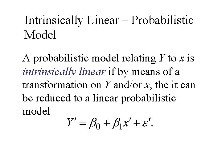
Intrinsically Linear – Probabilistic Model A probabilistic model relating Y to x is intrinsically linear if by means of a transformation on Y and/or x, the it can be reduced to a linear probabilistic model

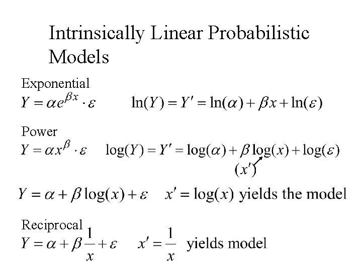
Intrinsically Linear Probabilistic Models Exponential Power Reciprocal

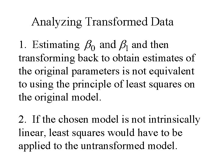
Analyzing Transformed Data 1. Estimating and then transforming back to obtain estimates of the original parameters is not equivalent to using the principle of least squares on the original model. 2. If the chosen model is not intrinsically linear, least squares would have to be applied to the untransformed model.

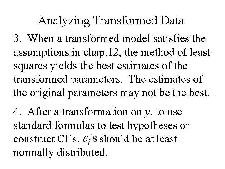
Analyzing Transformed Data 3. When a transformed model satisfies the assumptions in chap. 12, the method of least squares yields the best estimates of the transformed parameters. The estimates of the original parameters may not be the best. 4. After a transformation on y, to use standard formulas to test hypotheses or construct CI’s, should be at least normally distributed.

Analyzing Transformed Data 5. When y is transformed, the r 2 value from the resulting regression refers to variation in the explained by the transformation regression model.

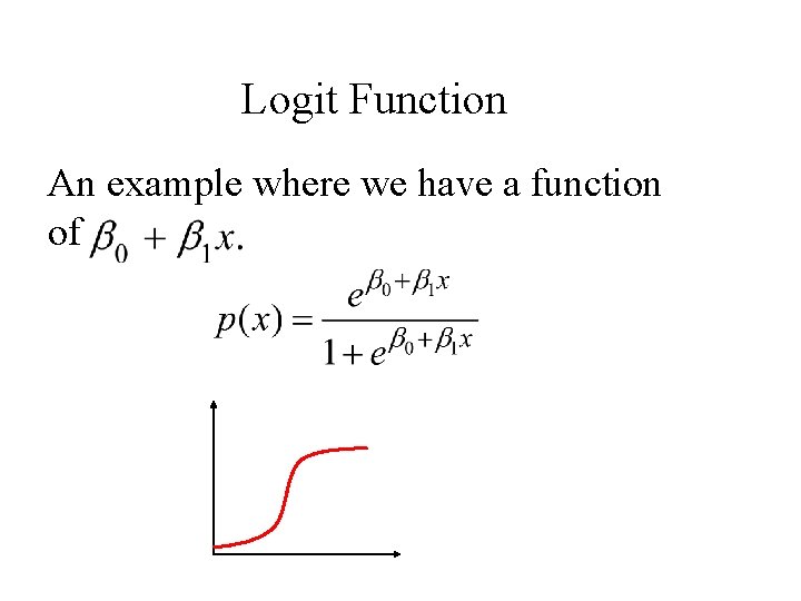
Logit Function An example where we have a function of

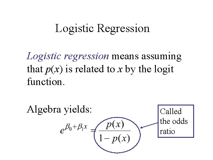
Logistic Regression Logistic regression means assuming that p(x) is related to x by the logit function. Algebra yields: Called the odds ratio

13. 3 Polynomial Regression

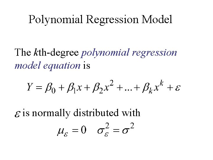
Polynomial Regression Model The kth-degree polynomial regression model equation is is normally distributed with

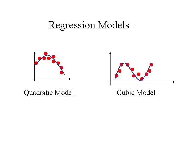
Regression Models Quadratic Model Cubic Model

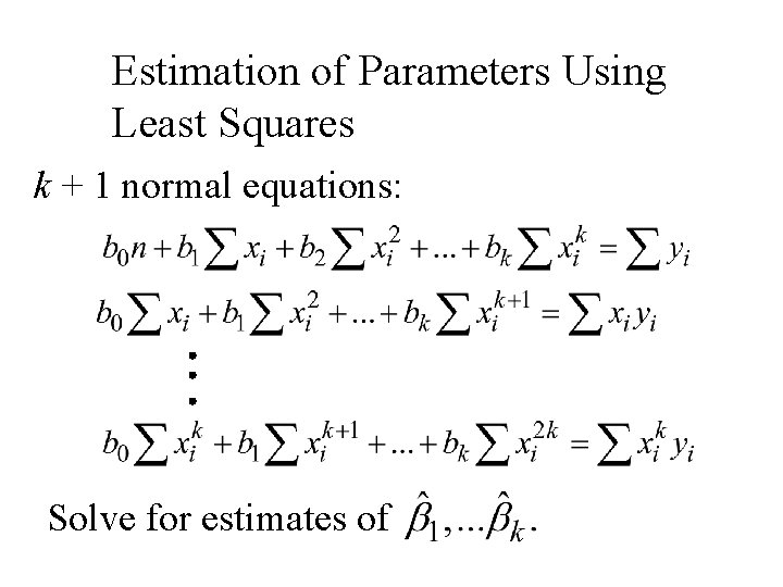
Estimation of Parameters Using Least Squares k + 1 normal equations: Solve for estimates of

Estimate of Coefficient of multiple determination: R 2 Adjusted R 2

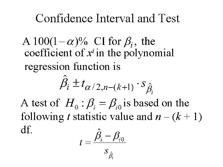
Confidence Interval and Test coefficient of xi in the polynomial regression function is A test of is based on the following t statistic value and n – (k + 1) df.

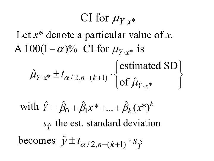
CI for Let x* denote a particular value of x. with becomes

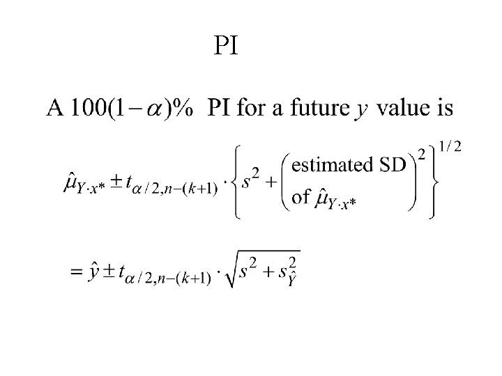
PI

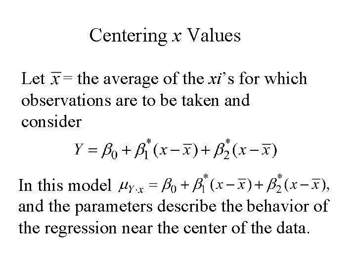
Centering x Values Let = the average of the xi’s for which observations are to be taken and consider In this model and the parameters describe the behavior of the regression near the center of the data.

13. 4 Multiple Regression Analysis

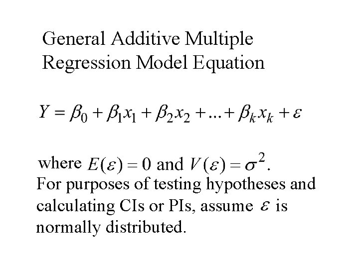
General Additive Multiple Regression Model Equation where For purposes of testing hypotheses and calculating CIs or PIs, assume is normally distributed.

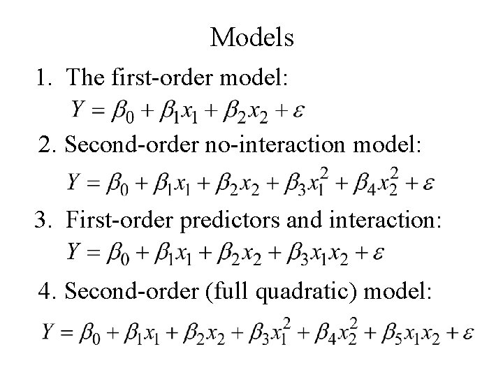
Models 1. The first-order model: 2. Second-order no-interaction model: 3. First-order predictors and interaction: 4. Second-order (full quadratic) model:

Models With Predictors for Categorical Variables Using simple numerical coding, qualitative (categorical) variables can be incorporated into a model. With a dichotomous variable associate an indicator (dummy) variable x whose possible values are 0 and 1.

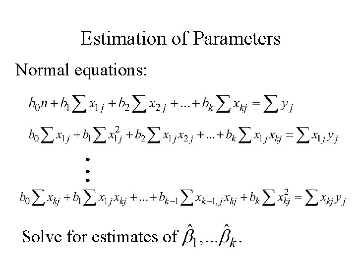
Estimation of Parameters Normal equations: Solve for estimates of

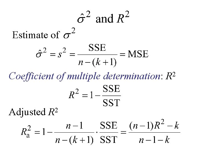
Estimate of Coefficient of multiple determination: R 2 Adjusted R 2

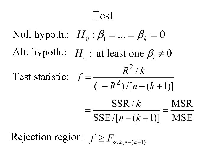
Test Null hypoth. : Alt. hypoth. : Test statistic: Rejection region:

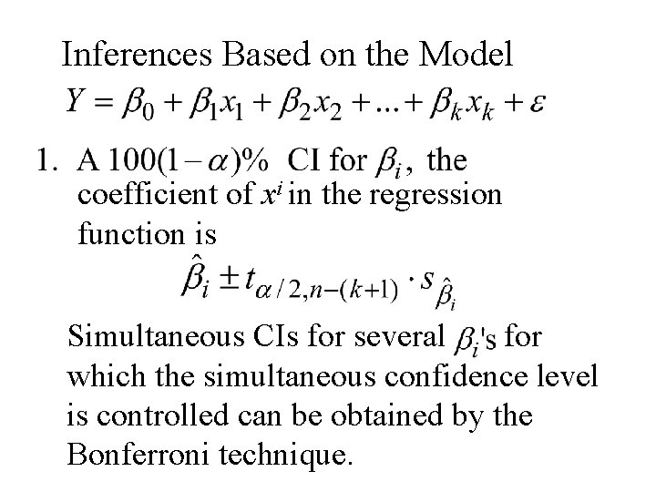
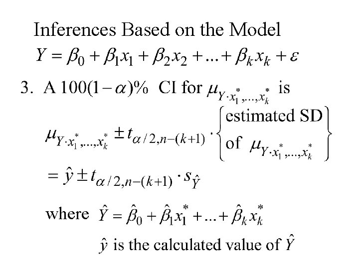
Inferences Based on the Model coefficient of xi in the regression function is Simultaneous CIs for several for which the simultaneous confidence level is controlled can be obtained by the Bonferroni technique.

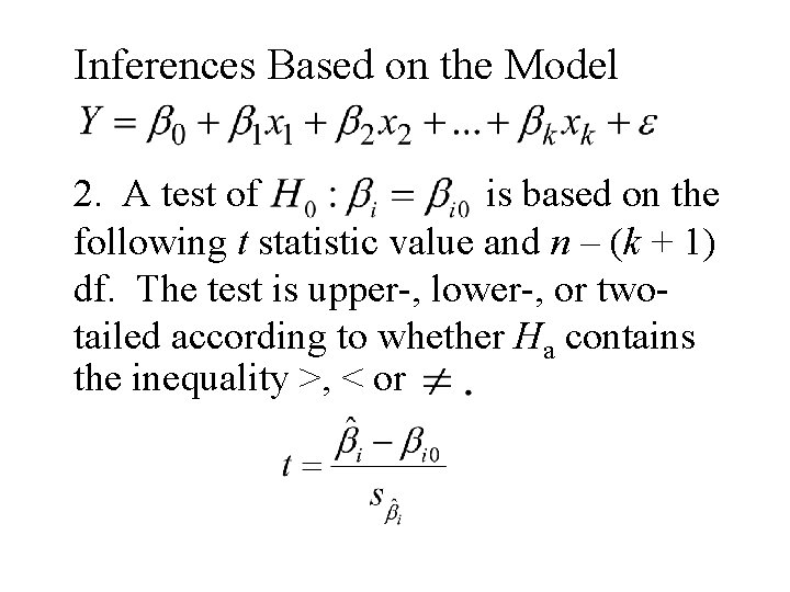
Inferences Based on the Model 2. A test of is based on the following t statistic value and n – (k + 1) df. The test is upper-, lower-, or twotailed according to whether Ha contains the inequality >, < or

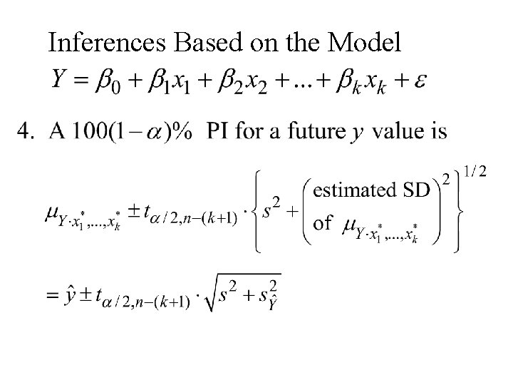
Inferences Based on the Model where

Inferences Based on the Model

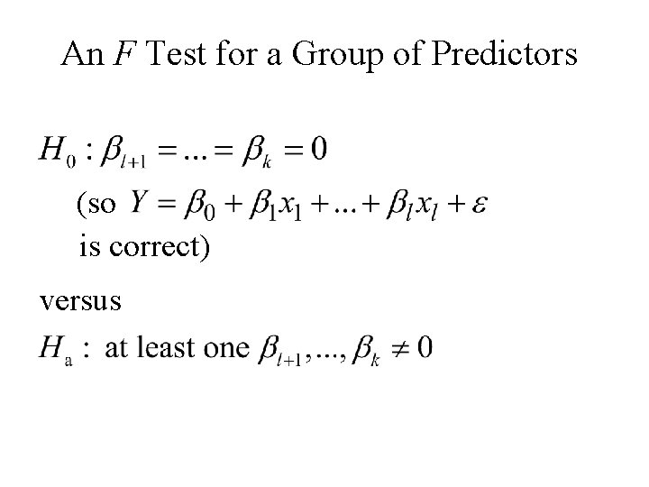
An F Test for a Group of Predictors (so is correct) versus

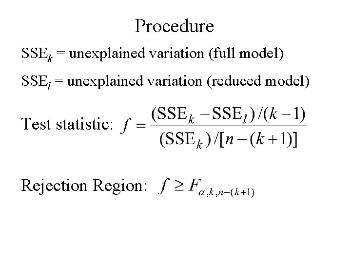
Procedure SSEk = unexplained variation (full model) SSEl = unexplained variation (reduced model) Test statistic: Rejection Region:

13. 5 Other Issues in Multiple Regression

Transformations in Multiple Regression Theoretical considerations or diagnostic plots may suggest a nonlinear relation between a dependent variable and two or more independent variables. Frequently a transformation will linearize the model.

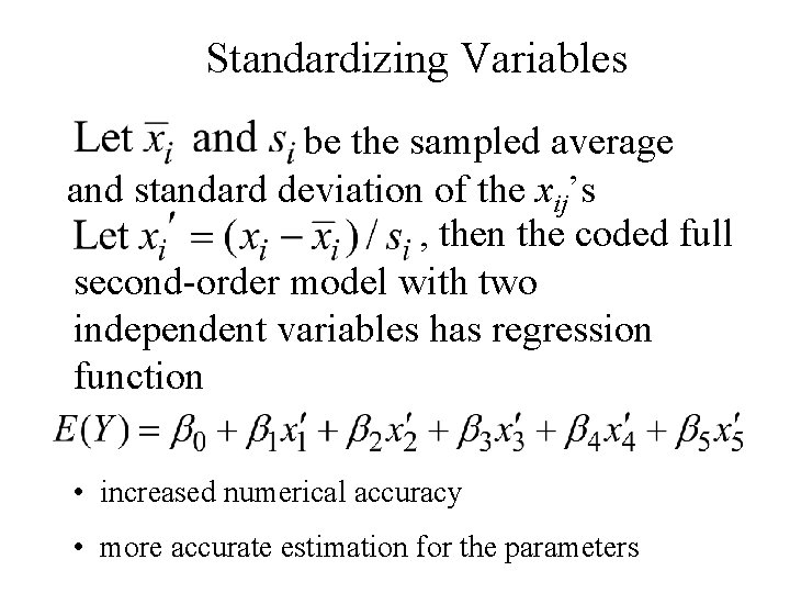
Standardizing Variables be the sampled average and standard deviation of the xij’s , then the coded full second-order model with two independent variables has regression function • increased numerical accuracy • more accurate estimation for the parameters

Variable Selection 1. If we examine regressions involving all possible subsets of the predictors for which data is available, what criteria should be used to select a model? 2. If the number of predictors is too large to examine all regressions, can a good model be found by examining a reduced number of subsets?

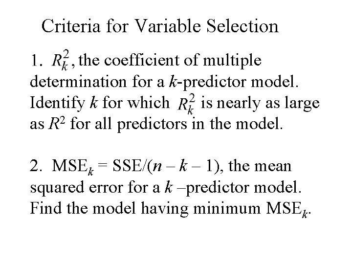
Criteria for Variable Selection the coefficient of multiple determination for a k-predictor model. Identify k for which is nearly as large as R 2 for all predictors in the model. 2. MSEk = SSE/(n – k – 1), the mean squared error for a k –predictor model. Find the model having minimum MSEk.

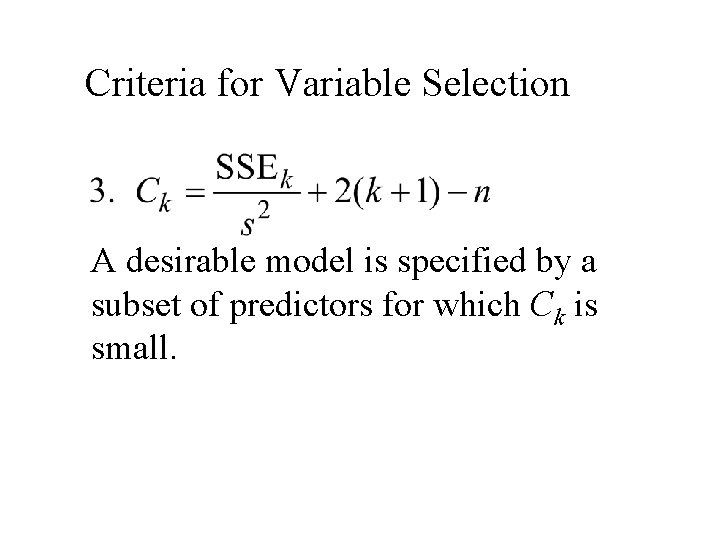
Criteria for Variable Selection A desirable model is specified by a subset of predictors for which Ck is small.

Stepwise Regression When the number of predictors is too large to allow for explicit or implicit examination of all possible subsets, alternative selection procedures generally identify good models. Two of these methods are the backward elimination (BE) method and the forward selection method (FS).

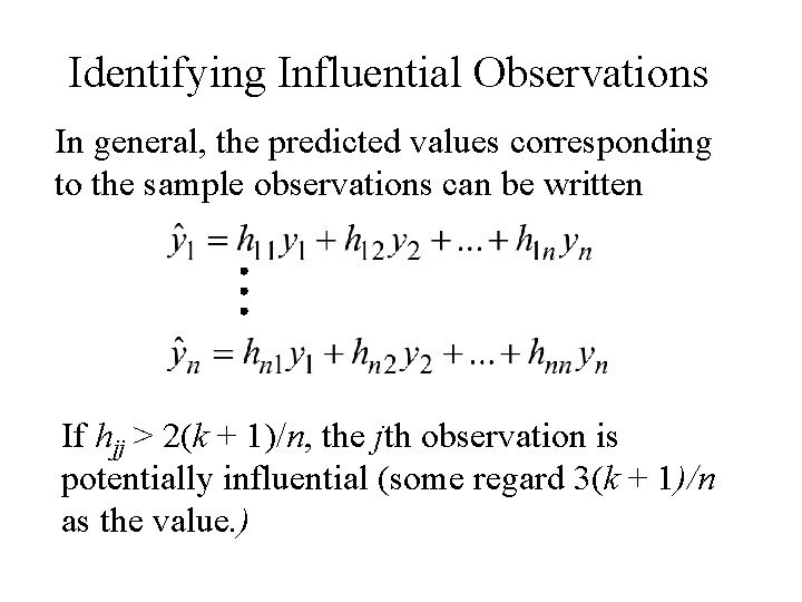
Identifying Influential Observations In general, the predicted values corresponding to the sample observations can be written If hjj > 2(k + 1)/n, the jth observation is potentially influential (some regard 3(k + 1)/n as the value. )