9 1 In1 matplotlib inline import numpy as

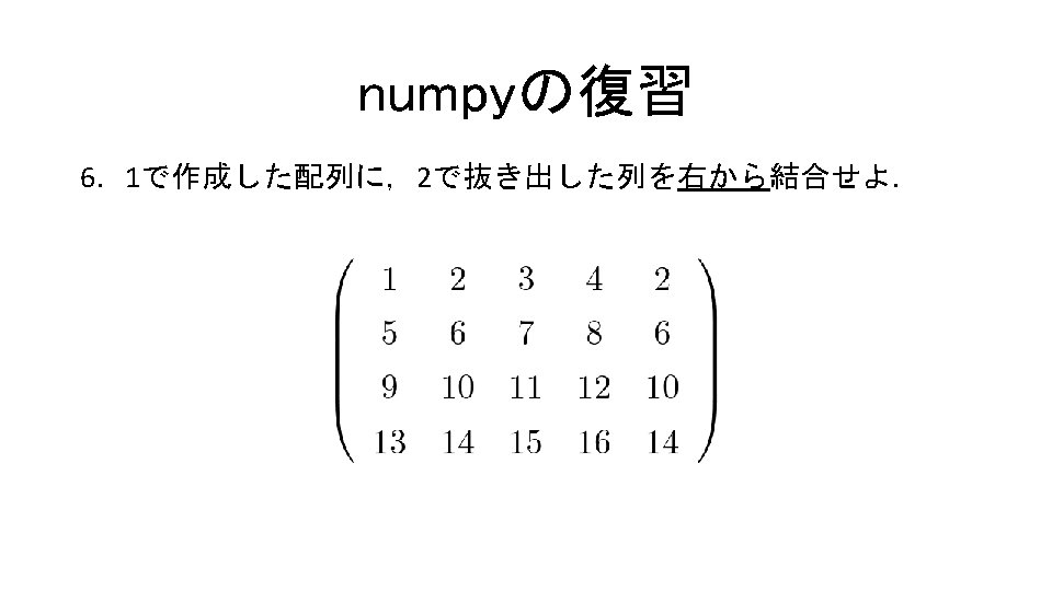
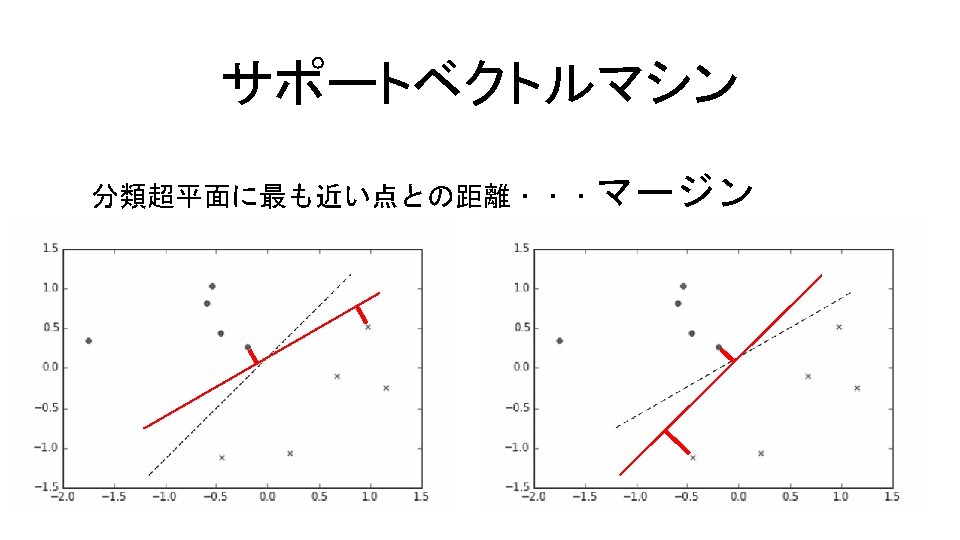
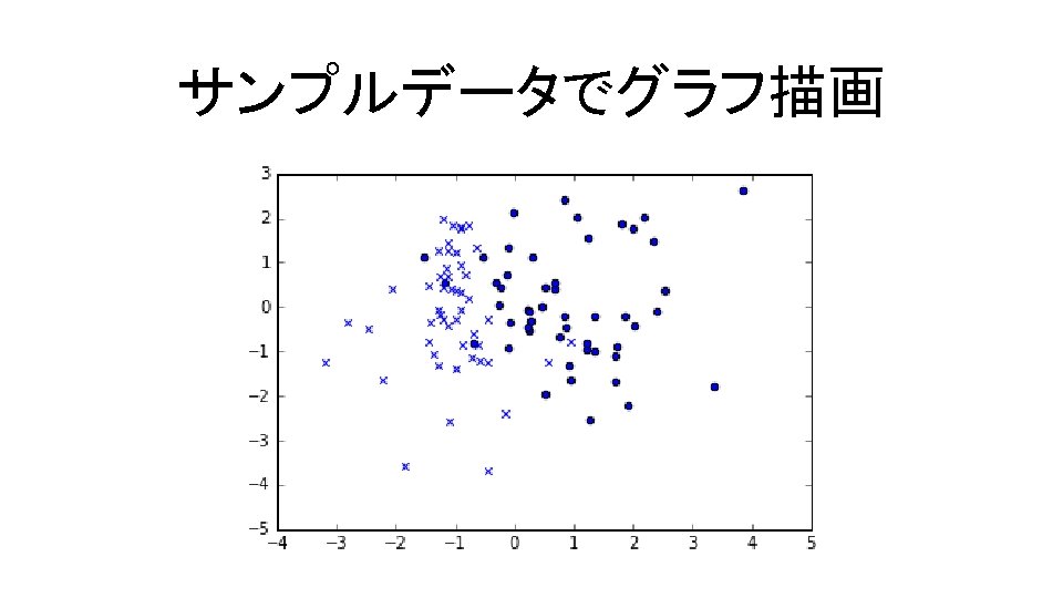
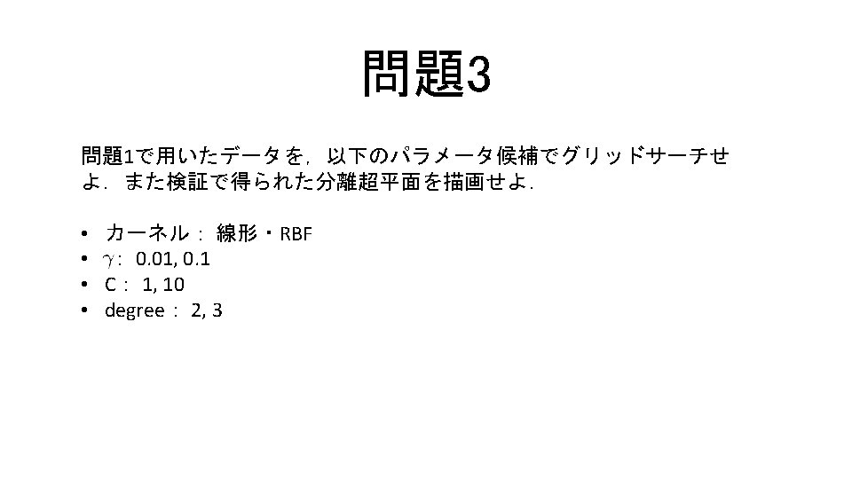
サンプルデータでグラフ描画 コード9. 1 In[1] %matplotlib inline import numpy as np import scipy. linalg as linalg from sklearn. datasets import * import matplotlib. pyplot as plt import sklearn. svm as svm np. random. seed(0) X, Y = make_classification(n_features=2, n_redundant=0, n_informative=2) iy = (Y == 1) iny = (Y == 0) plt. scatter(X[iy, 0], X[iy, 1], marker='o') plt. scatter(X[iny, 0], X[iny, 1], marker='x');

サンプルデータでグラフ描画 X, Y = make_classification(n_features=2, n_redundant=0, n_informative=2) X >>>array([[ -7. 66054695 e-01, 1. 83324682 e-01], [ -9. 20383253 e-01, -7. 23168038 e-02], [ -9. 86585088 e-01, -2. 86920000 e-01], [ 1. 70910242 e+00, -1. 10453952 e+00], [ 1. 98764670 e+00, 1. 77624479 e+00], [ 3. 86274219 e+00, 2. 63325914 e+00], [ -1. 12836011 e+00, -4. 22761581 e-01], [ -1. 10074198 e+00, -2. 56042975 e+00], 　　　� サンプルデータ

サンプルデータでグラフ描画 X, Y = make_classification(n_features=2, n_redundant=0, n_informative=2) Y >>>array([0, 1, 1, 1, 0, 0, 1, 1, 1, 0, 1, 0, 1, 1, 0, 0, 0, 1, 0, 1, 1, 1, 0, 0, 0, 1, 1, 0]) 1, 1, 0, 0, 1, 1, 1, 0, 0, 1, 0, 1, 1, 0, 0, 1, 1, 0, 1, 0, 0, 1, 1, 0, n_classesがデフォルトの 2　　　2種類に特徴づけられている ラベルデータ 0, 0, 0, 1, 0, 1, 0, 1, 1, 1, 0, 1,

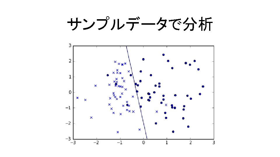
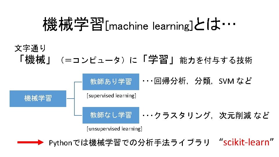
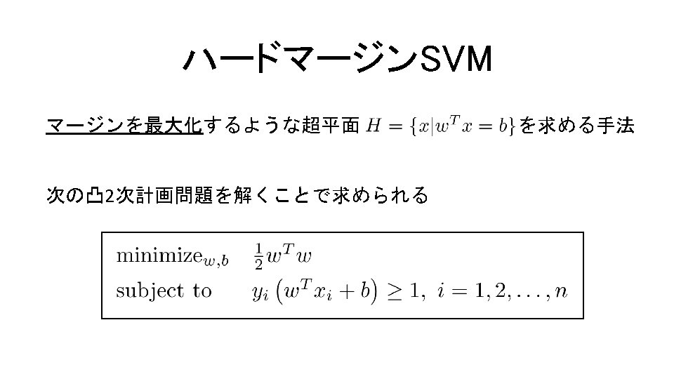
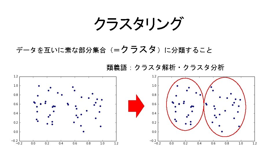
サンプルデータで分析 コード9. 2 In[2] clf = svm. SVC(kernel='linear', C=1. 0) clf. fit(X, Y) カーネル関数を指定 （デフォルトはrbf） Support Vector Classification fit … SVCモデルをデータに適応する ペナルティ項の係数を指定 （デフォルトが1. 0） コード9. 2 Out[2] SVC(C=1. 0, cache_size=200, class_weight=None, coef 0=0. 0, decision_function_shape=None, degree=3, gamma='auto', kernel='linear', max_iter=-1, probability=False, random_state=None, shrinking=True, tol=0. 001, verbose=False)

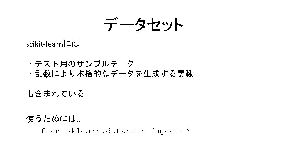
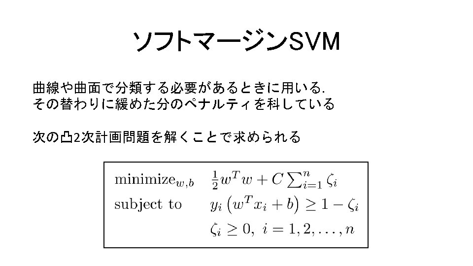
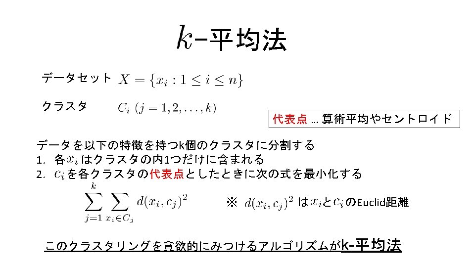
サンプルデータで分析 領域をメッシュに区切り，グリッド上で決定関数=0の等高線を描く コード9. 3 In[3] xx, yy = np. meshgrid(np. linspace(-3, 3, 500), np. linspace(-3, 3, 500)) Z = clf. decision_function(np. c_[xx. ravel(), yy. ravel()]) Z = Z. reshape(xx. shape) ctr = plt. contour(xx, yy, Z, levels=[0], linetypes='--') plt. scatter(X[iy, 0], X[iy, 1], marker='o') plt. scatter(X[iny, 0], X[iny, 1], marker='x') plt. axis([xx. min(), xx. max(), yy. min(), yy. max()]) plt. show() ravel … フラットなarrayに変換する． decision_function … 分離超平面の決定関数を返す

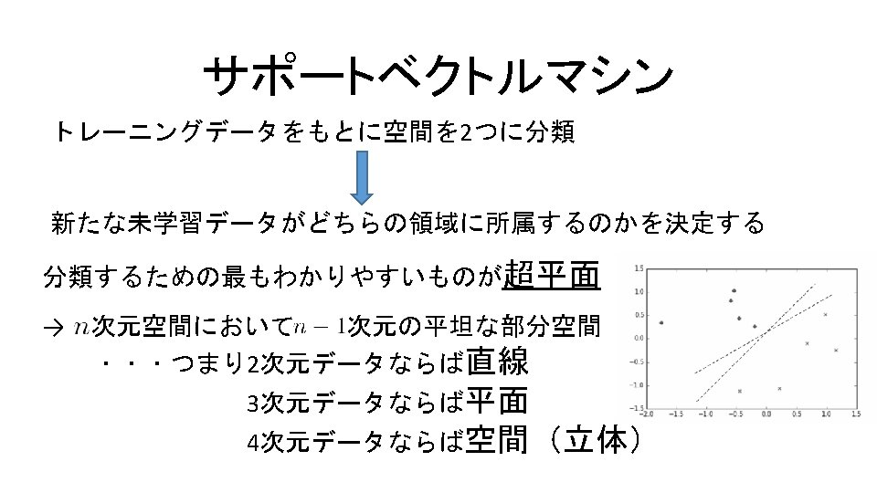
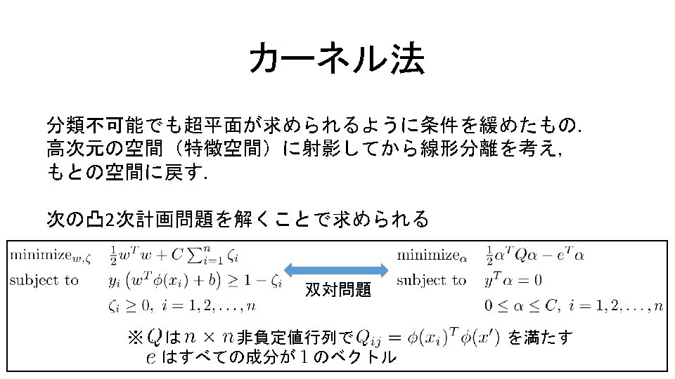
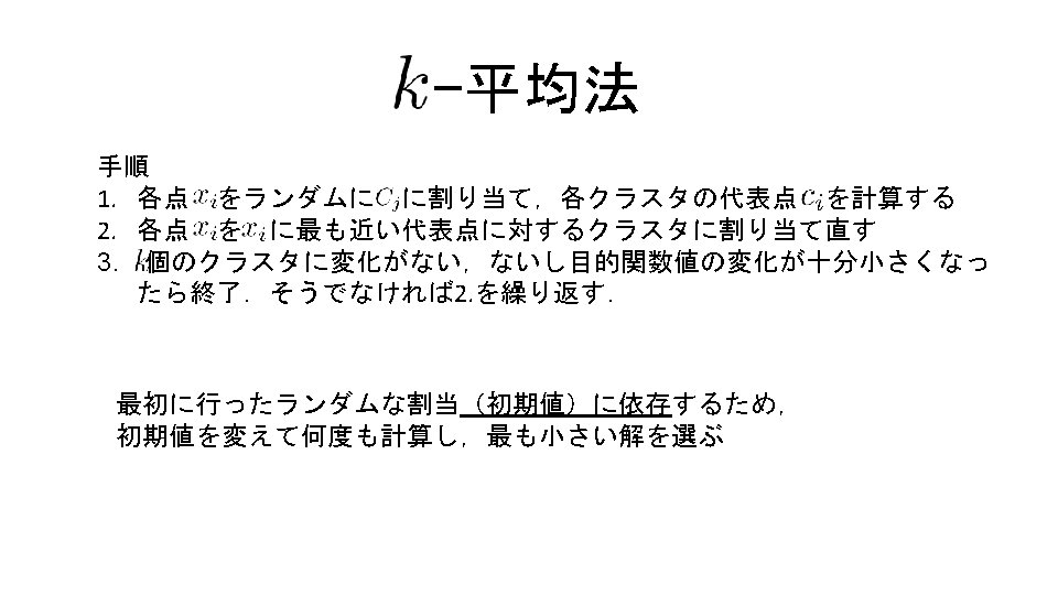
サポートベクトル回帰 コード9. 4 In[4] import numpy as np import matplotlib. pyplot as plt # 学習データ作成 np. random. seed(1000) n = 50 x = np. sort(np. random. uniform(-np. pi, n)) y = np. sin(x)+np. random. randn(n)*0. 2 plt. plot(x, y, 'o'); このデータに線形，RBF，多項式カーネル のサポートベクトル回帰を行う

サポートベクトル回帰 コード9. 5 In[6] Support Vector # モデルの定義 svr_rbf = svm. SVR(kernel='rbf', C=1000, gamma=0. 1) svr_lin = svm. SVR(kernel='linear', C=1000) svr_poly = svm. SVR(kernel='poly', C=1000, degree=3) # 分析 X = x. reshape(-1, 1) y_rbf = svr_rbf. fit(X, y). predict(X) y_lin = svr_lin. fit(X, y). predict(X) y_poly = svr_poly. fit(X, y). predict(X) Regression reshape(1, -1) … 2次元横ベクトル reshape(-1, 1) … 2次元縦ベクトル predict … データの回帰を実行

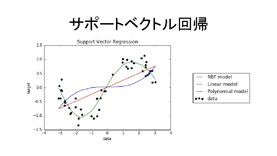
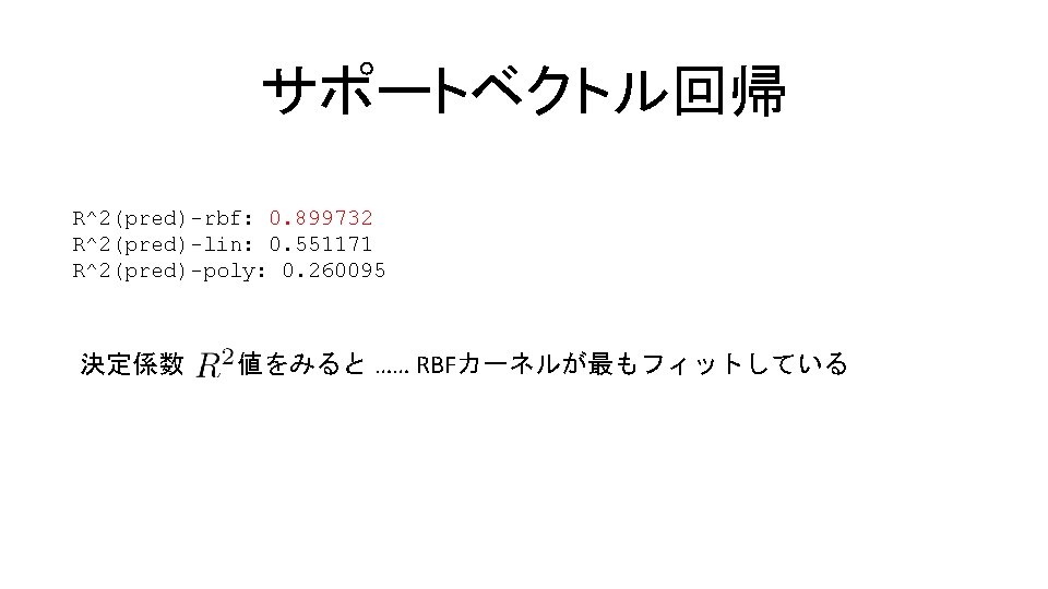
サポートベクトル回帰 コード9. 5 In[6] # 結果のグラフ化 plt. scatter(x, y, c='k', label='data') plt. plot(x, y_rbf, c='g', label='RBF model') plt. plot(x, y_lin, c='r', label='Linear model') plt. plot(x, y_poly, c='b', label='Polynomial model') plt. xlabel('data') plt. ylabel('target') plt. title('Support Vector Regression') plt. legend(loc='upper center', bbox_to_anchor=(1. 4, 0. 7)) plt. show() # 分析結果 print('R^2(pred)-rbf: %f' % svm. SVR. score(svr_rbf, X, y)) print('R^2(pred)-lin: %f' % svm. SVR. score(svr_lin, X, y)) print('R^2(pred)-poly: %f' % svm. SVR. score(svr_poly, X, y))

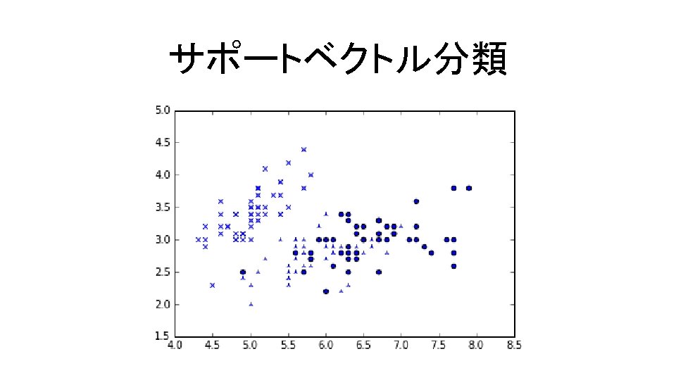
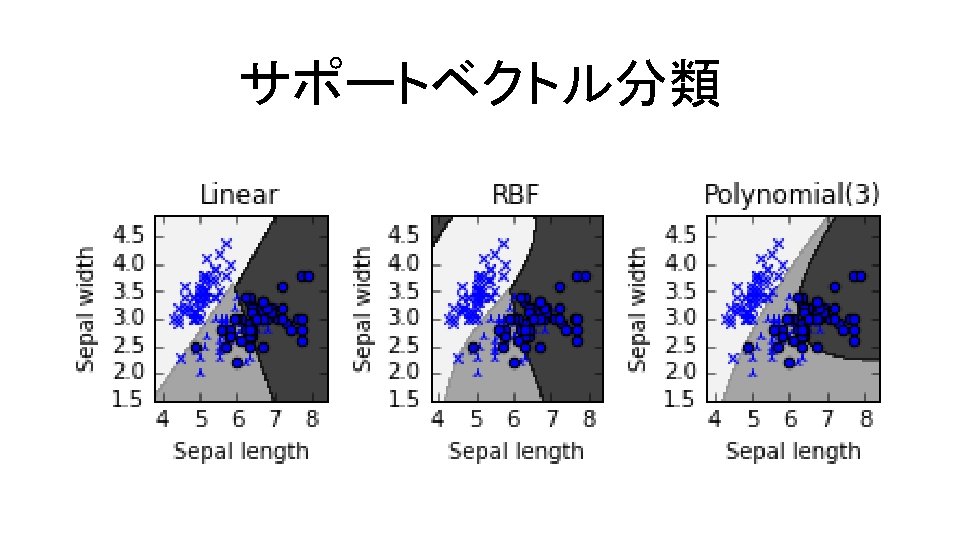
サポートベクトル分類 3種類のアヤメの花の萼片の長さと幅，花弁の長さと幅についてのデータ を使って，多クラスの分類を行う コード9. 6 In[7] import numpy as np import matplotlib. pyplot as plt from sklearn import svm, datasets iris = datasets. load_iris() X = iris. data[: , 0: 2] y = iris. target load_iris … アヤメの花に関するデータ読込 iy 0 = (y == 0); iy 1 = (y == 1); iy 2 = (y == 2) plt. scatter(X[iy 0, 0], X[iy 0, 1], marker='x') plt. scatter(X[iy 1, 0], X[iy 1, 1], marker='2') plt. scatter(X[iy 2, 0], X[iy 2, 1], marker='o');

サポートベクトル分類 コード9. 7 In[8] C = 1. 0 Support svc_lin = svm. SVC(kernel='linear', C=C); svc_lin. fit(X, y) svc_rbf = svm. SVC(kernel='rbf', gamma=1. 0, C=C); svc_rbf. fit(X, y) svc_poly = svm. SVC(kernel='poly', degree=3, C=C); svc_poly. fit(X, y) Vector Classification irisデータに線形・RBF・多項式カーネルの 3つを適用して分類

サポートベクトル分類 コード9. 8 In[9] x_min, x_max = X[: , 0]. min() - 0. 5, X[: , 0]. max() + 0. 5 for i, clf in enumerate((svc_lin, svc_rbf, svc_poly)): plt. subplot(2, 3, i +1) y_min, y_max = X[: , 1]. min() - 0. 5, X[: , 1]. max() + 0. 5 plt. subplots_adjust(wspace=0. 6, hspace=0. 6) xx, yy = np. meshgrid(np. linspace(x_min, x_max, 300), np. linspace(y_min, y_max, 300)) Z = clf. predict(np. c_[xx. ravel(), yy. ravel()]) # タイトル titles = ['Linear', 'RBF', 'Polynomial(3)'] Z = Z. reshape(xx. shape) plt. contourf(xx, yy, Z, cmap='binary', alpha=0. 8) plt. scatter(X[iy 0, 0], X[iy 0, 1], marker='x') plt. scatter(X[iy 1, 0], X[iy 1, 1], marker='2') plt. scatter(X[iy 2, 0], X[iy 2, 1], marker='o') plt. xlabel('Sepal length') plt. ylabel('Sepal width') plt. xlim(xx. min(), xx. max()) plt. ylim(yy. min(), yy. max()) plt. title(titles[i])

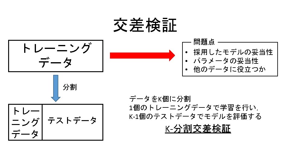
交差検証 コード9. 9 In[10] # 交差検証 from sklearn. cross_validation import cross_val_score print('訓練誤差: ') for i, clf in enumerate((svc_lin, svc_rbf, svc_poly)): print(u'%s Kernel での訓練誤差: %f ' % (titles[i], clf. score(X, y))) cv = cross_val_score(clf, X, y, cv=3) print(u' 交差検証でのスコア: ', cv) cross_val_score … モデルの評価を行う 　　cvはデータを何分割するか

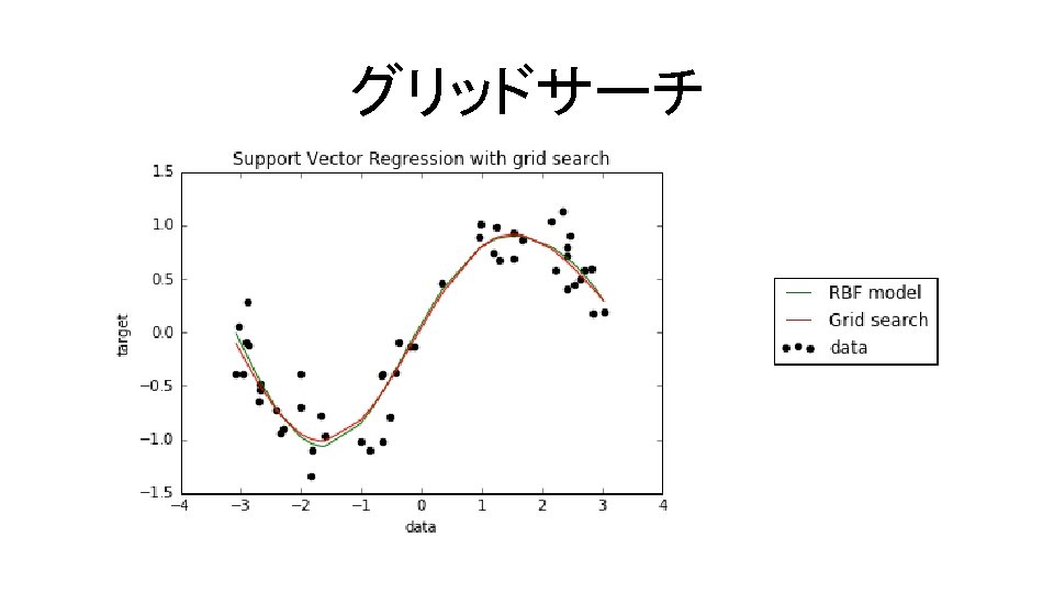
グリッドサーチ 交差検証を用いてモデル（カーネル）選定，パラメータ設定を行う コード9. 10 In[11] from sklearn. grid_search import Grid. Search. CV params = [{'kernel': ['rbf', 'poly'], 'gamma': [0. 01, 0. 1], 'C': [1, 10], 'degree': [2, 3]}] gscv = Grid. Search. CV(svm. SVR(), params, cv=5) gscv. fit(X, y) print(gscv. best_estimator_) print(gscv. best_score_) print(gscv. best_params_) カーネルやパラメータの 候補を自分で設定する

グリッドサーチ SVR(C=10, cache_size=200, coef 0=0. 0, degree=2, epsilon=0. 1, gamma=0. 1, kernel='rbf', max_iter=-1, shrinking=True, tol=0. 001, verbose=False) 0. 00332049460486 {'gamma': 0. 1, 'C': 10, 'degree': 2, 'kernel': 'rbf'} ※教科書の例と候補が異なるので， 教科書の出力と同一の出力にはならないので注意

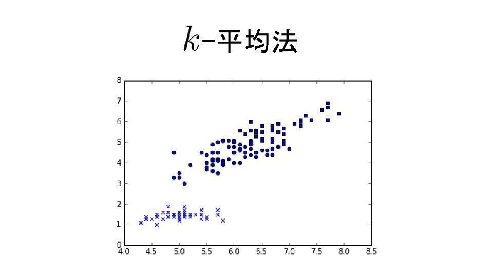
-平均法 コード9. 11 In[12] %matplotlib inline from matplotlib. pyplot import * import sklearn. datasets, sklearn. cluster # irisデータの読込 d = sklearn. datasets. load_iris() print(d. DESCR) 最適化を何度実行するか コード9. 12 In[13] km = sklearn. cluster. KMeans(n_clusters=3, init='random', n_jobs=10) km. fit(d. data) for i, e in enumerate(d. data): scatter(e[0], e[2], marker='xos'[km. labels_[i]])

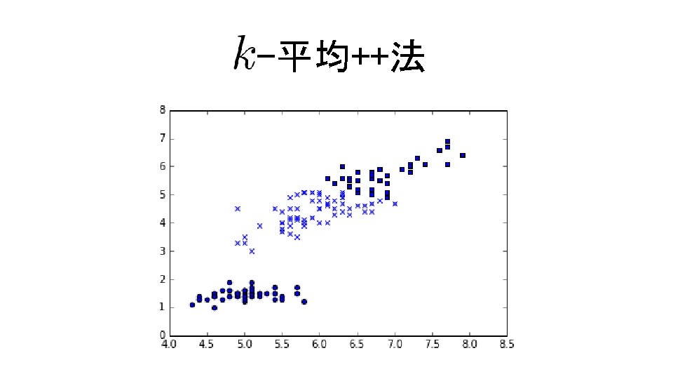
　 -平均++法 コード9. 12 In[13] km = sklearn. cluster. KMeans(n_clusters=3, init='random', n_jobs=10) km. fit(d. data) for i, e in enumerate(d. data): scatter(e[0], e[2], marker='xos'[km. labels_[i]]) コード9. 13 In[14] km = sklearn. cluster. KMeans(n_clusters=3, init='k-means++', n_jobs=10) km. fit(d. data) for i, e in enumerate(d. data): scatter(e[0], e[2], marker='xos'[km. labels_[i]])

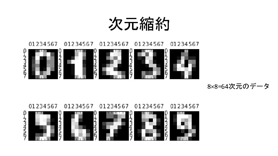
コード9. 14 In[15] 次元縮約 # モジュールの読み込み %matplotlib inline import sklearn. datasets, sklearn. decomposition, sklearn. metrics from sklearn. svm import Linear. SVC import matplotlib. pyplot as plt import numpy as np # 画像データの読込 d = sklearn. datasets. load_digits() 0 -9のアラビア数字の手書 き文字のデジタルデータ print('データの数: %d' % len(d. data)) print('0 番目の画像データに関する情報') print(d. target[0]) print(d. data[0]) print(d. images[0]) plt. gray() # colorマップをグレースケールにして画像を出力 for i in range(10): plt. subplot(2, 5, i+1) plt. matshow(d. images[i], 0)

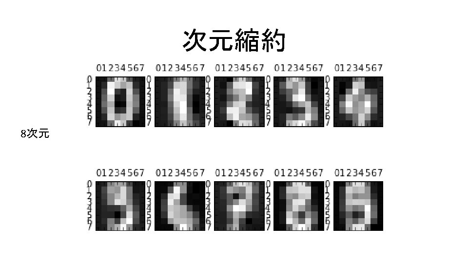
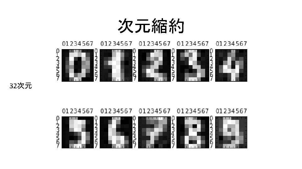
次元縮約 コード9. 15 In[16] pca = sklearn. decomposition. PCA(32) # モデル指定。次元は３２ 。 r = pca. fit_transform(d. data) # 次元削減を実行。結果をr に。 rd = pca. inverse_transform(r) # rをもとの 64 次元に戻し、 # 画像を描画 for i in range(10): plt. subplot(2, 5, i+1) plt. matshow(rd[i]. reshape(8, 8), 0) PCA … 主成分分析のモデル fit_transform … 次元削減を適用する inverse_transform … データを元の空間に戻 す

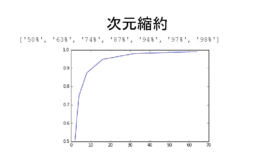
次元縮約 客観的に次元削減を評価する関数もある コード9. 16 In[17] res, rng = [], [2, 3, 4, 8, 16, 32, 64] for i in rng: pca = sklearn. decomposition. PCA(i) r = pca. fit_transform(d. data) svc = Linear. SVC() svc. fit(r, d. target) res. append(sklearn. metrics. accuracy_score(svc. predict(r), d. target)) print([str(int(i*100))+'%' for i in res]) plt. plot(rng, res); accuracy_score … 分類精度の評価を行う