The Squared Correlation 2 r What Does It

The Squared Correlation 2 r – What Does It Tell Us? Lecture 51 Sec. 13. 9 Tue, May 2, 2006

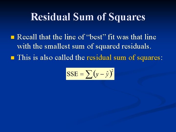
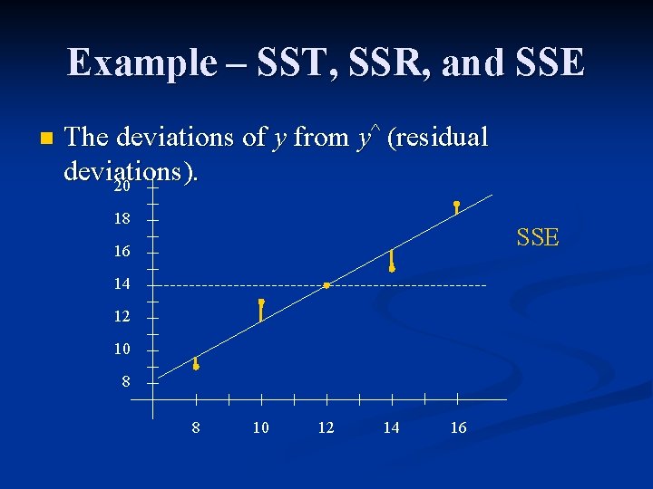
Residual Sum of Squares Recall that the line of “best” fit was that line with the smallest sum of squared residuals. n This is also called the residual sum of squares: n

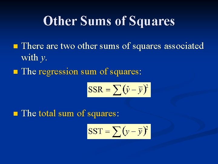
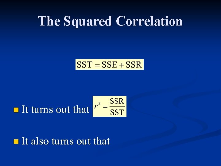
Other Sums of Squares There are two other sums of squares associated with y. n The regression sum of squares: n n The total sum of squares:

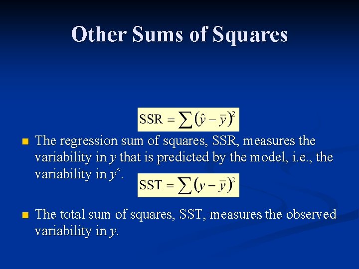
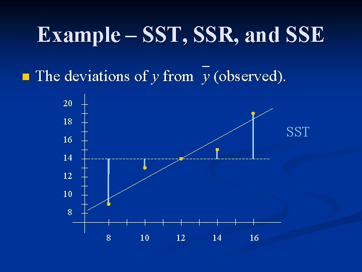
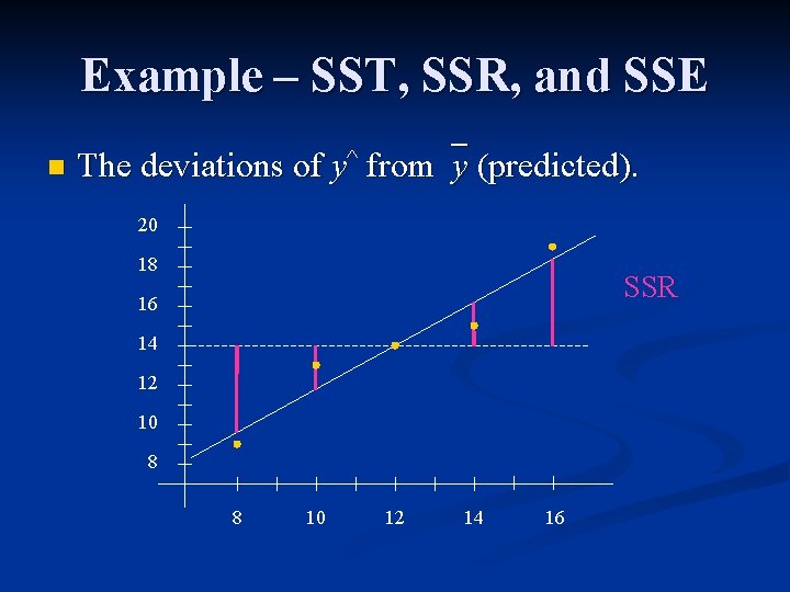
Other Sums of Squares n The regression sum of squares, SSR, measures the variability in y that is predicted by the model, i. e. , the variability in y^. n The total sum of squares, SST, measures the observed variability in y.

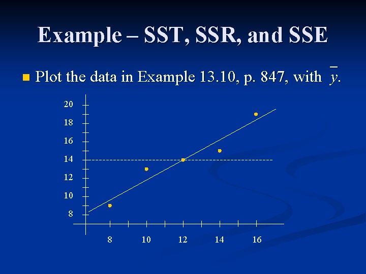
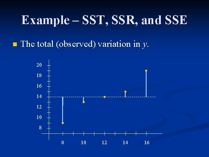
Example – SST, SSR, and SSE n Plot the data in Example 13. 10, p. 847, with y. 20 18 16 14 12 10 8 8 10 12 14 16

Example – SST, SSR, and SSE n The deviations of y from y (observed). 20 18 SST 16 14 12 10 8 8 10 12 14 16

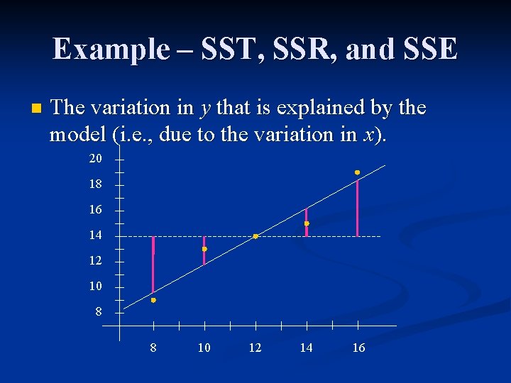
Example – SST, SSR, and SSE n The deviations of y^ from y (predicted). 20 18 SSR 16 14 12 10 8 8 10 12 14 16

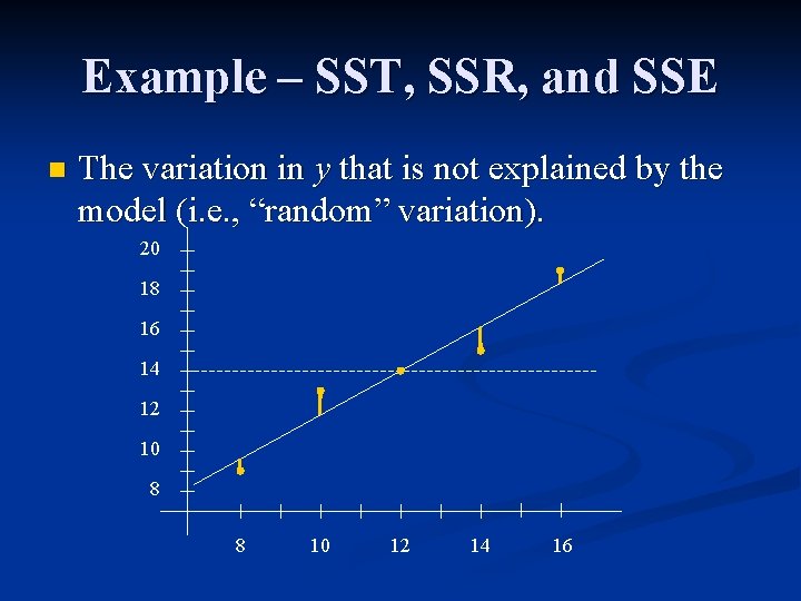
Example – SST, SSR, and SSE n The deviations of y from y^ (residual deviations). 20 18 SSE 16 14 12 10 8 8 10 12 14 16

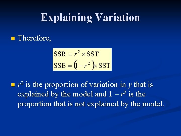
The Squared Correlation n It turns out that n It also turns out that

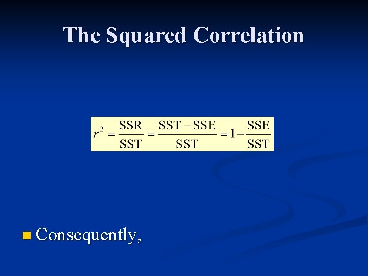
The Squared Correlation n Consequently,

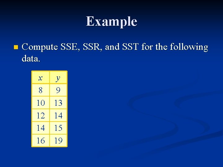
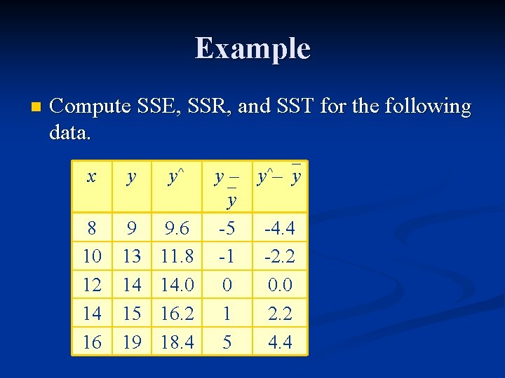
Example n Compute SSE, SSR, and SST for the following data. x 8 10 12 14 16 y 9 13 14 15 19

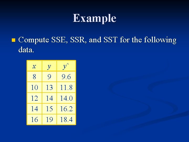
Example n Compute SSE, SSR, and SST for the following data. x 8 10 12 14 16 y 9 13 14 15 19 y^ 9. 6 11. 8 14. 0 16. 2 18. 4

Example n Compute SSE, SSR, and SST for the following data. x y y^ 8 10 12 14 16 9 13 14 15 19 9. 6 11. 8 14. 0 16. 2 18. 4 y – y^– y y -5 -4. 4 -1 -2. 2 0 0. 0 1 2. 2 5 4. 4

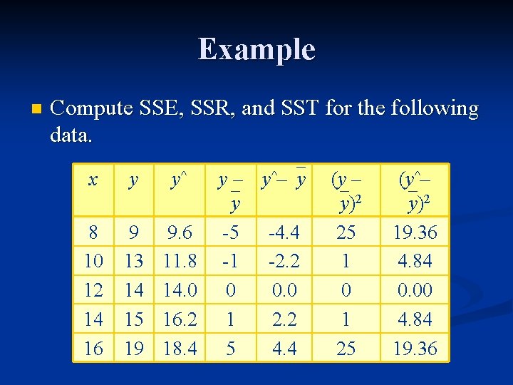
Example n Compute SSE, SSR, and SST for the following data. x y y^ 8 10 12 14 16 9 13 14 15 19 9. 6 11. 8 14. 0 16. 2 18. 4 y – y^– y y -5 -4. 4 -1 -2. 2 0 0. 0 1 2. 2 5 4. 4 (y – y)2 25 1 0 1 25 (y^– y)2 19. 36 4. 84 0. 00 4. 84 19. 36

Example n Compute SSE, SSR, and SST for the following data. x y y^ 8 10 12 14 15 9 13 14 15 19 9. 6 11. 8 14. 0 16. 2 18. 4 y – y^– y y -5 -4. 4 -1 -2. 2 0 0. 0 1 2. 2 5 4. 4 (y – y)2 25 1 0 1 25 52 (y^– y)2 19. 36 4. 84 0. 00 4. 84 19. 36 48. 40

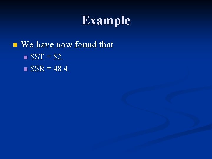
Example n We have now found that SST = 52. n SSR = 48. 4. n

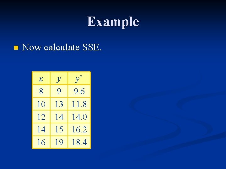
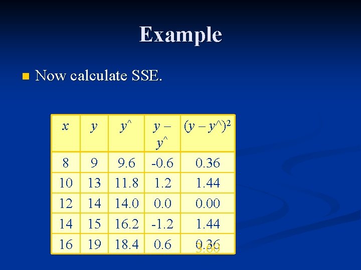
Example n Now calculate SSE. x 8 10 12 14 16 y 9 13 14 15 19 y^ 9. 6 11. 8 14. 0 16. 2 18. 4

Example n Now calculate SSE. x y y^ 8 10 12 14 16 9 13 14 15 19 9. 6 11. 8 14. 0 16. 2 18. 4 y – (y – y^)2 y^ -0. 6 0. 36 1. 2 1. 44 0. 00 -1. 2 1. 44 0. 6 0. 36

Example n Now calculate SSE. x y y^ 8 10 12 14 16 9 13 14 15 19 9. 6 11. 8 14. 0 16. 2 18. 4 y – (y – y^)2 y^ -0. 6 0. 36 1. 2 1. 44 0. 00 -1. 2 1. 44 0. 6 0. 36 3. 60

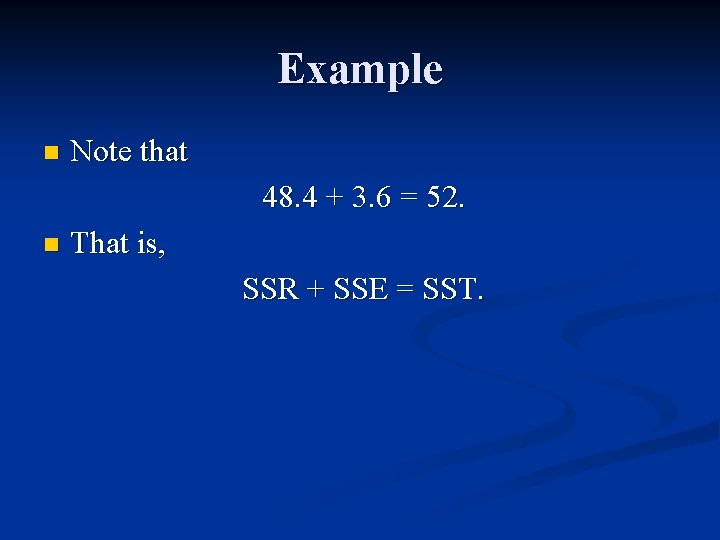
Example n Note that 48. 4 + 3. 6 = 52. n That is, SSR + SSE = SST.

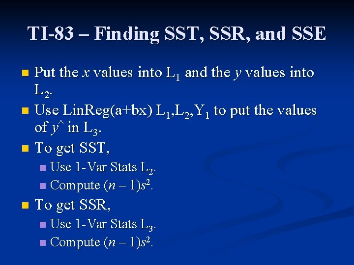
TI-83 – Finding SST, SSR, and SSE Put the x values into L 1 and the y values into L 2. n Use Lin. Reg(a+bx) L 1, L 2, Y 1 to put the values of y^ in L 3. n To get SST, n Use 1 -Var Stats L 2. n Compute (n – 1)s 2. n n To get SSR, Use 1 -Var Stats L 3. n Compute (n – 1)s 2. n

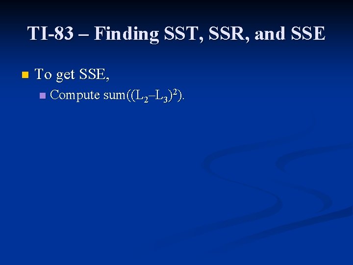
TI-83 – Finding SST, SSR, and SSE n To get SSE, n Compute sum((L 2–L 3)2).

Explaining Variation One goal of regression is to “explain” the variation in y. n For example, if x were height and y were weight, how would we explain the variation in weight? n n n That is, why do some people weigh more than others? Or if x were the hours spent studying for a math test and y were the score on the test, how would we explain the variation in scores? n That is, why do some people score higher than

Explaining Variation n A certain amount of the variation in y can be explained by the variation in x. Some people weigh more than others because they are taller. n Some people score higher on math tests because they studied more. n n But that is never the full explanation. Not all taller people weigh more. n Not everyone who studies more scores higher. n

Explaining Variation High degree of correlation between x and y variation in x explains most of the variation in y. n Low degree of correlation between x and y variation in x explains only a little of the variation in y. n In other words, the amount of variation in y that is explained by the variation in x should be related to r. n

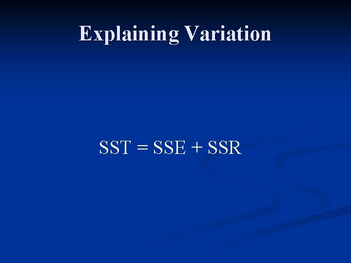
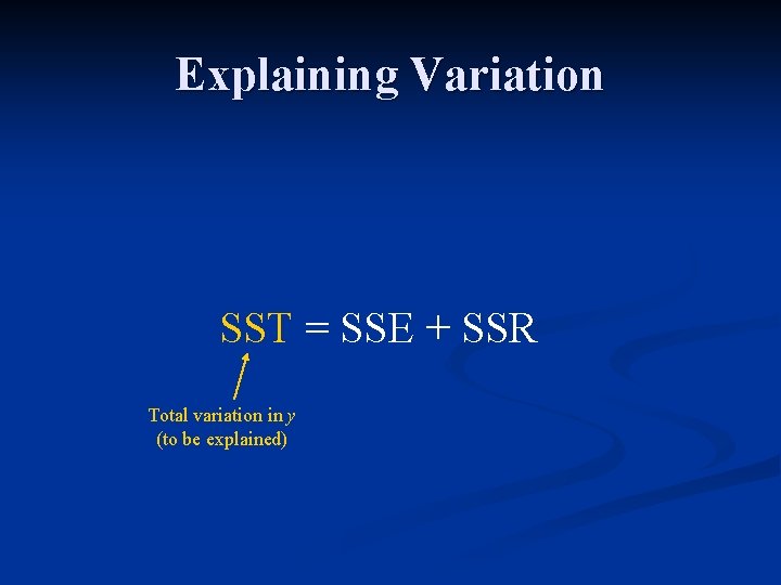
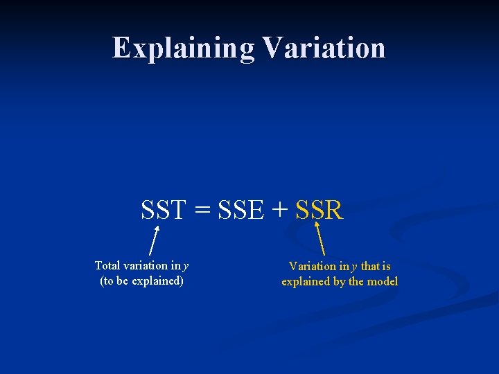
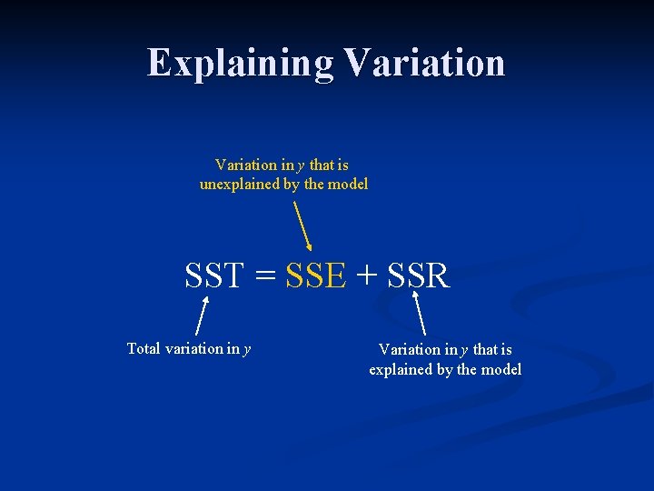
Explaining Variation Statisticians consider the predicted variation SSR to be the amount of variation in y (i. e. , SST) that is explained by the model. n The remaining variation in y, i. e. , the residual variation SSE, is the amount that is not explained by the model. n

Explaining Variation SST = SSE + SSR

Explaining Variation SST = SSE + SSR Total variation in y (to be explained)

Explaining Variation SST = SSE + SSR Total variation in y (to be explained) Variation in y that is explained by the model

Explaining Variation in y that is unexplained by the model SST = SSE + SSR Total variation in y Variation in y that is explained by the model

Example – SST, SSR, and SSE n The total (observed) variation in y. 20 18 16 14 12 10 8 8 10 12 14 16

Example – SST, SSR, and SSE n The variation in y that is explained by the model (i. e. , due to the variation in x). 20 18 16 14 12 10 8 8 10 12 14 16

Example – SST, SSR, and SSE n The variation in y that is not explained by the model (i. e. , “random” variation). 20 18 16 14 12 10 8 8 10 12 14 16

Explaining Variation n Therefore, n r 2 is the proportion of variation in y that is explained by the model and 1 – r 2 is the proportion that is not explained by the model.

TI-83 – Calculating r 2 n To calculate r 2 on the TI-83, Follow the procedure that produces the regression line and r. n In the same window, the TI-83 reports r 2. n