Synthesis of Unit Hydrographs for Texas Watersheds Theodore

Synthesis of Unit Hydrographs for Texas Watersheds Theodore G. Cleveland, UH William H. Asquith, USGS David B. Thompson, R. O. Anderson Xing Fang, Auburn University July 17, 2007

Acknowledgements • Research colleagues: – Meghan Roussel, USGS – Amanda Garcia, USGS – George R. Herrmann, Tx. DOT • Funding: – Texas Department of Transportation • 0 -4193, 0 -4194, 0 -4696, 0 -5822

Research Context • Unit hydrograph (UH) methods are used to: – Obtain peak discharge and hydrograph shape for drainage design. – Compute a direct runoff hydrograph for a particular storm event when applied in conjunction with a hyetograph and rainfall-runoff model – Analyze complex problems in integrated arrangements of sub-watersheds which are combined using routing technology (e. g. HEC-HMS, HEC-RAS, SWMM). • Typically used: – Drainage areas too large for rational methods. – For drainage areas small enough for lumped-parameter model.

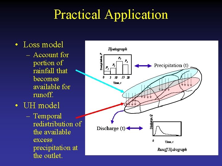
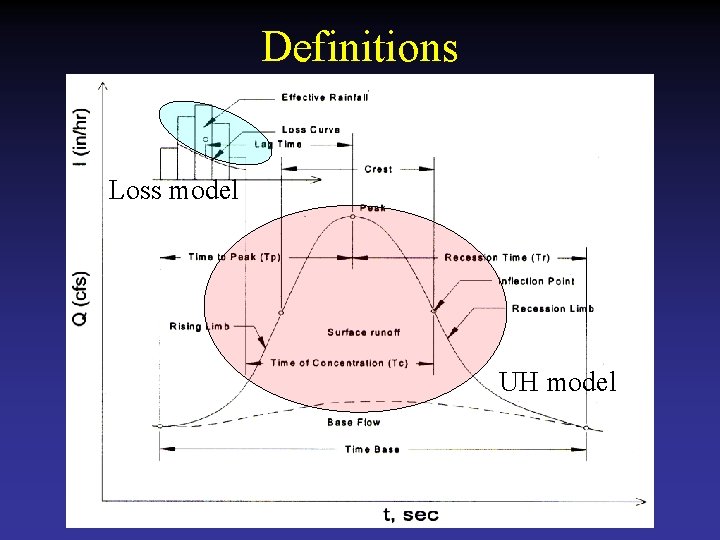
Practical Application • Loss model – Account for portion of rainfall that becomes available for runoff. • UH model – Temporal redistribution of the available excess precipitation at the outlet.

Definitions • Loss Models – The “equation” that converts precipitation to excess precipitation; it does NOT redistribute the signal in time. • • • Proportional loss model Phi-index Initial Abstraction - Constant Rate NRCS CN Infiltration capacity (e. g. Green-Ampt)

Definitions • UH Model – The “equation” that redistributes the excess precipitation the signal in time to the outlet. • Discrete unit hydrographs (e. g. Sherman) • Gamma-family unit hydrographs • Geomorphic unit hydrographs.

Definitions Loss model UH model

Definitions • Characteristic Times – Time-to-peak • Time from inception of runoff to peak discharge value. Often used as a parameter in hydrograph models. – Time-of-concentration • Time required for parcel of water to travel from the most distant (hydrologic) point in a watershed to the outlet.

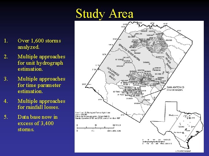
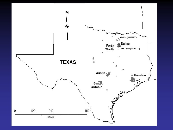
Study Area 1. Over 1, 600 storms analyzed. 2. Multiple approaches for unit hydrograph estimation. 3. Multiple approaches for time parameter estimation. 4. Multiple approaches for rainfall losses. 5. Data base now in excess of 3, 400 storms.

Research Approaches • Multiple lines of research – Discrete Unit Graphs • Analyst directed and automated • Multiple regression for regionalization. – Gamma Unit Graph • Analyst directed • Multiple regression for regionalization. – Geomorphic Instantaneous Unit Graph (GIUH) • Automated • Independent comparison.

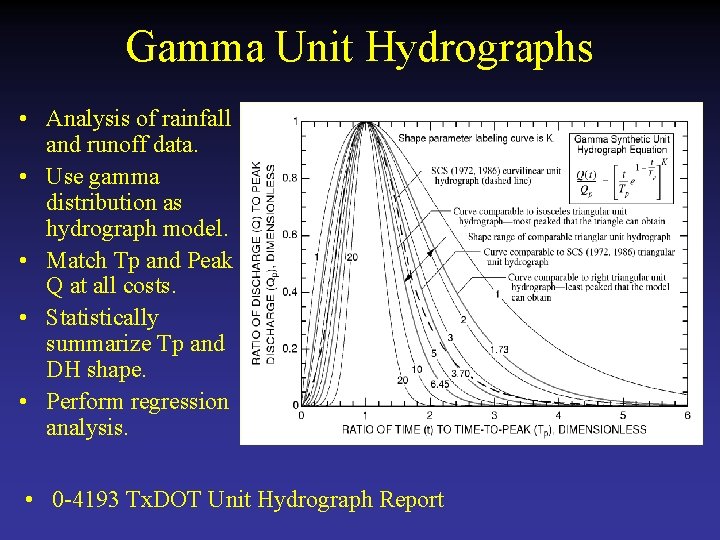
Gamma Unit Hydrographs • Analysis of rainfall and runoff data. • Use gamma distribution as hydrograph model. • Match Tp and Peak Q at all costs. • Statistically summarize Tp and DH shape. • Perform regression analysis. • 0 -4193 Tx. DOT Unit Hydrograph Report

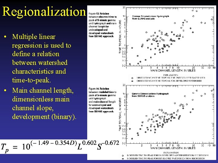
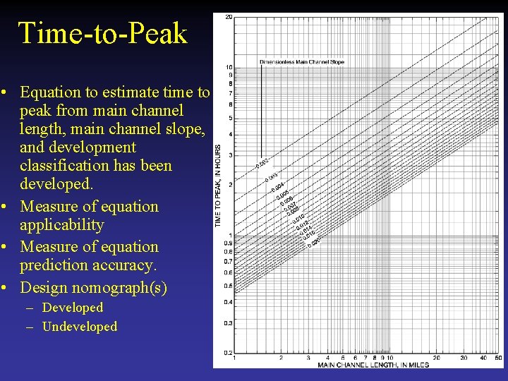
Regionalization • Multiple linear regression is used to define a relation between watershed characteristics and time-to-peak. • Main channel length, dimensionless main channel slope, development (binary).

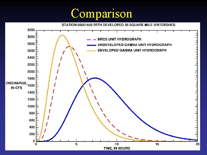
Comparison

Time-to-Peak • Equation to estimate time to peak from main channel length, main channel slope, and development classification has been developed. • Measure of equation applicability • Measure of equation prediction accuracy. • Design nomograph(s) – Developed – Undeveloped

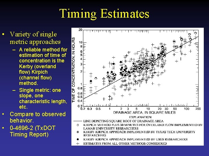
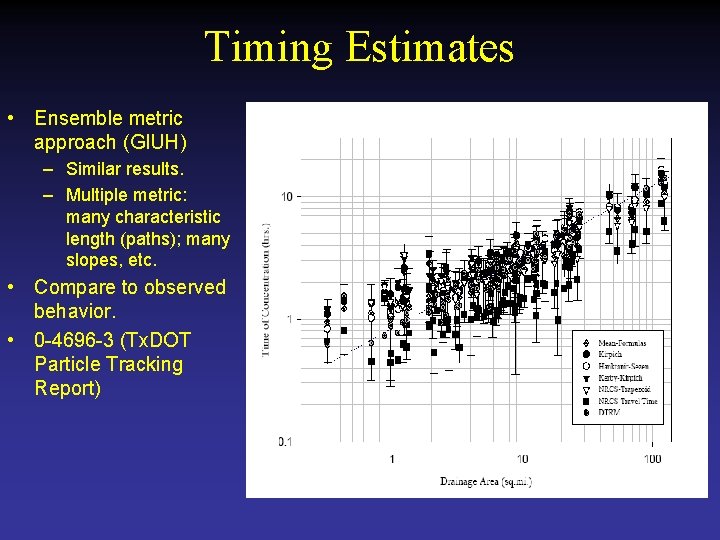
Timing Estimates • Variety of single metric approaches – A reliable method for estimation of time of concentration is the Kerby (overland flow) Kirpich (channel flow) method. – Single metric: one slope, one characteristic length, etc. • Compare to observed behavior. • 0 -4696 -2 (Tx. DOT Timing Report)

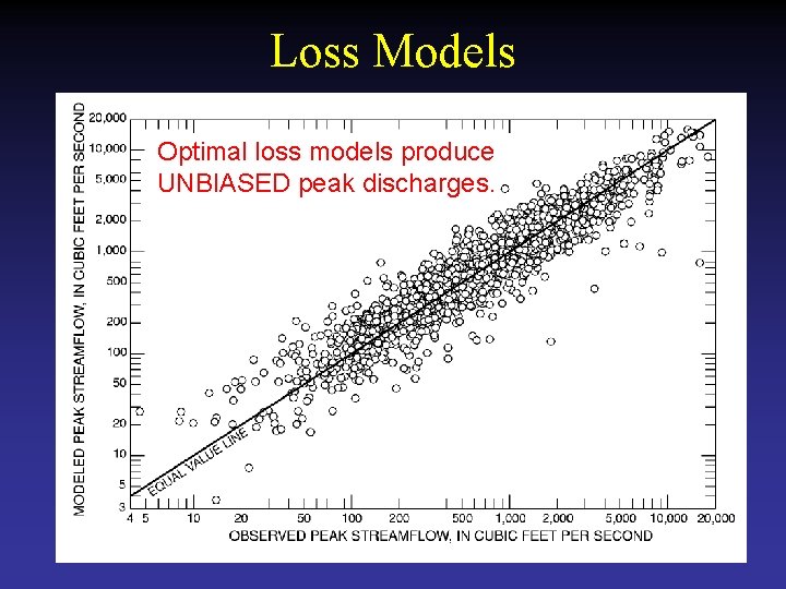
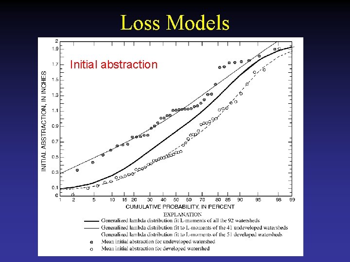
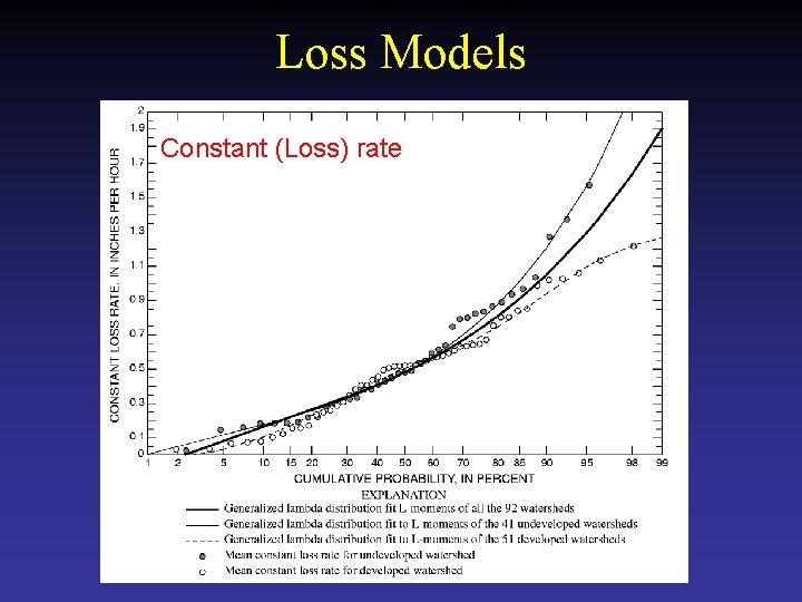
Loss Models • Let us use that UH with real rainfall to estimate the parameters of an initial abstraction-constant loss model. • Estimate those loss-model parameters through optimization by constraining the parameters to realistic values, constraining the optimization to volume match, and minimizing on the residuals of the modeled and observed hydrographs.

Loss Models Optimal loss models produce UNBIASED peak discharges.

Loss Models Initial abstraction

Loss Models Constant (Loss) rate

Geomorphic IUH Approach • Timing values are property of physical characteristics. – Same as regression approach. – Same as other approaches. • Ensemble of properties extracted from DEM raster (paths, slopes along paths, etc. ) – Set of metrics instead of a single metric.

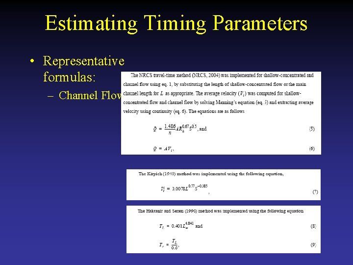
Estimating Timing Parameters • Representative formulas: – Channel Flow

Estimating Timing Parameters • The formulas beg the questions: – Which “lengths, slopes, friction factors” ? – What is “bankful discharge” on an ungaged watershed ? – Which “paths” to examine ?

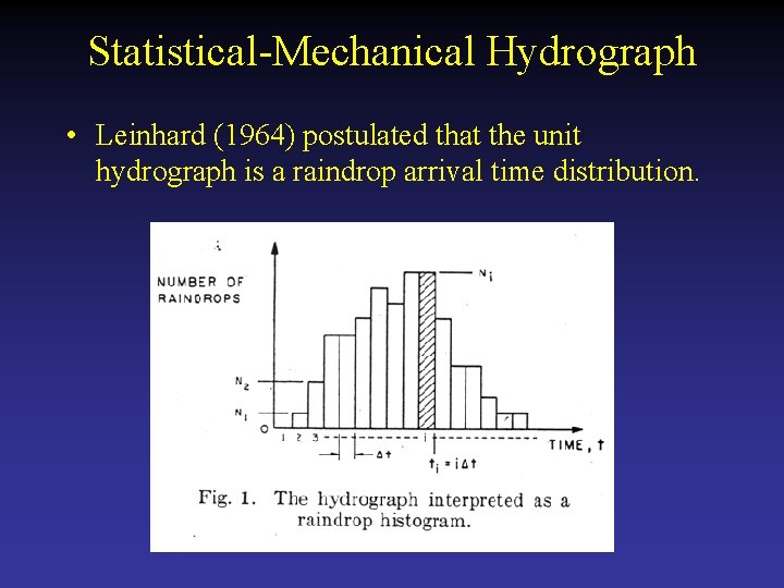
Statistical-Mechanical Hydrograph • Leinhard (1964) postulated that the unit hydrograph is a raindrop arrival time distribution.

Statistical-Mechanical Hydrograph • Further Assumed: – The arrival time of a raindrop is proportional to the distance it must travel, l. – The number of drops arriving at the outlet in a time interval is proportional to the square of travel time (and l 2 ). – By enumerating all possible arrival time histograms, and selecting the most probable from maximum likelihood arrived at a probability distribution that represents the temporal redistribution of rainfall on the watershed.

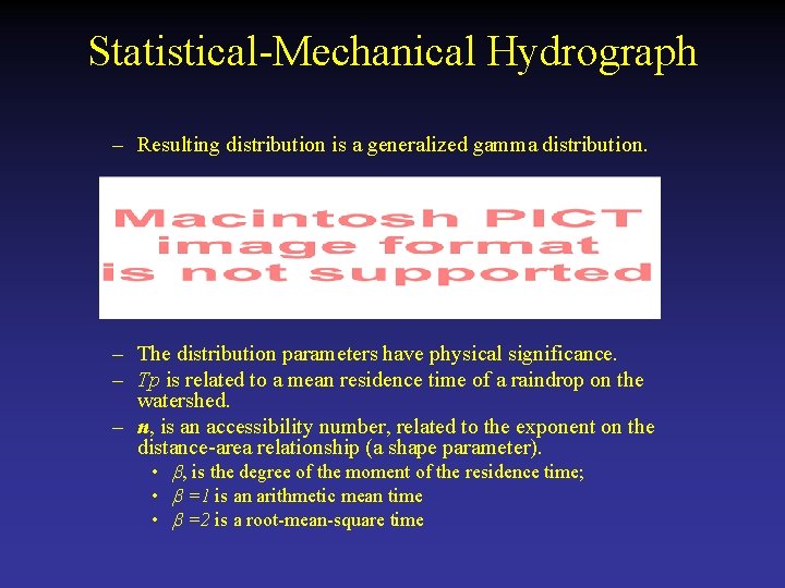
Statistical-Mechanical Hydrograph – Resulting distribution is a generalized gamma distribution. – The distribution parameters have physical significance. – Tp is related to a mean residence time of a raindrop on the watershed. – n, is an accessibility number, related to the exponent on the distance-area relationship (a shape parameter). • b, is the degree of the moment of the residence time; • b =1 is an arithmetic mean time • b =2 is a root-mean-square time

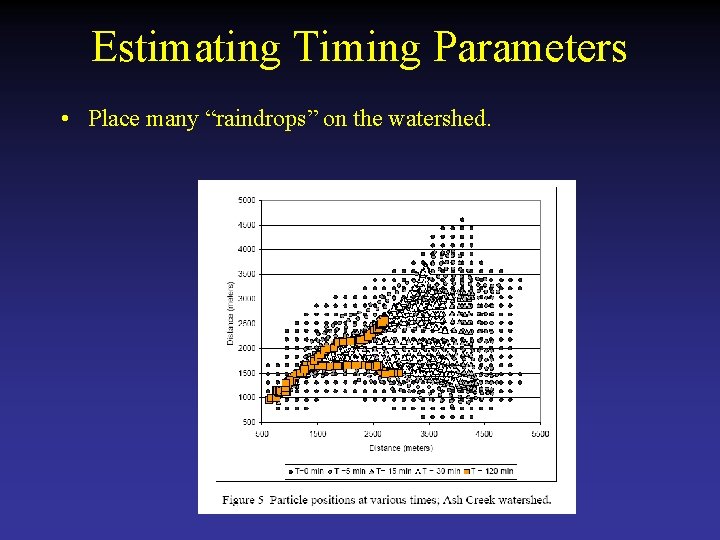
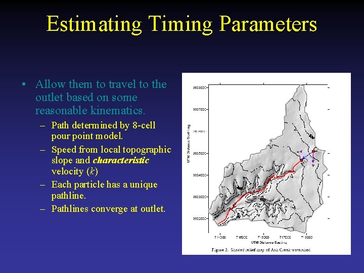
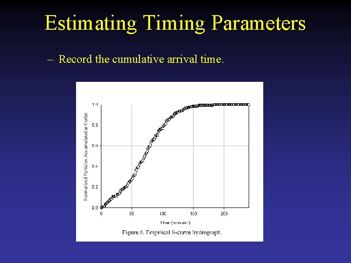
Estimating Timing Parameters • The derivation based on enumeration suggests an algorithm to approximate watershed behavior. – Place many “raindrops” on the watershed. – Allow them to travel to the outlet based on some reasonable kinematics. (Explained later - significant variable is a “k” term represents friction) – Record the cumulative arrival time. – Infer Tp and n from the cumulative arrival time distribution. – The result is an instantaneous unit hydrograph.

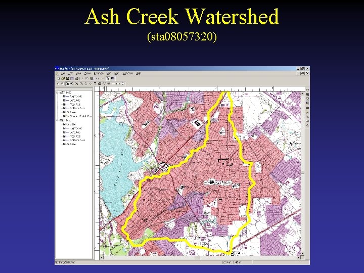
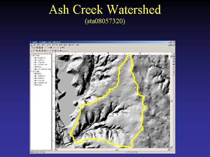
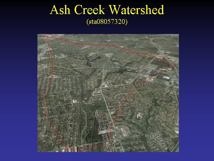
Estimating Timing Parameters • Illustrate with Ash Creek Watershed – Calibration watershed – the “k” term was selected by analysis of one storm on this watershed, and applied to all developed watersheds studied. – About 7 square miles. (20, 000+ different “paths”)

Ash Creek Watershed (sta 08057320)

Ash Creek Watershed (sta 08057320)

Ash Creek Watershed (sta 08057320)

Estimating Timing Parameters • Place many “raindrops” on the watershed.

Estimating Timing Parameters • Allow them to travel to the outlet based on some reasonable kinematics. – Path determined by 8 -cell pour point model. – Speed from local topographic slope and characteristic velocity (k) – Each particle has a unique pathline. – Pathlines converge at outlet.

Estimating Timing Parameters – Record the cumulative arrival time.

Estimating Timing Parameters – Infer Tp and n from the cumulative arrival time distribution.

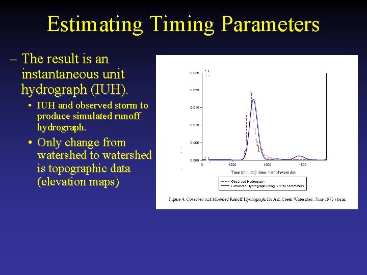
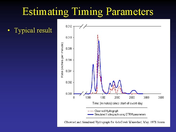
Estimating Timing Parameters – The result is an instantaneous unit hydrograph (IUH). • IUH and observed storm to produce simulated runoff hydrograph. • Only change from watershed to watershed is topographic data (elevation maps)

Parameterization • Need to know “k”. – Can make reasonable guess based on intuition: larger than zero, smaller than terminal velocity of a large water balloon; probably on the order of 100 -1000 feet/minute - but really have no clue. – Used a SINGLE storm in Dallas, adjust “k” to get good “match” - use this “k” for every other watershed without further adjustment.

Estimating Timing Parameters • Typical result

Timing Estimates • Ensemble metric approach (GIUH) – Similar results. – Multiple metric: many characteristic length (paths); many slopes, etc. • Compare to observed behavior. • 0 -4696 -3 (Tx. DOT Particle Tracking Report)

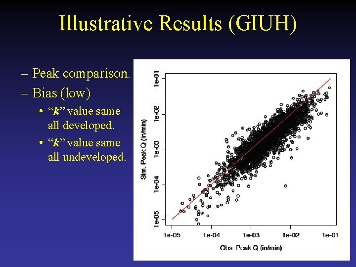
Illustrative Results (GIUH) – Peak comparison. – Bias (low) • “k” value same all developed. • “k” value same all undeveloped.

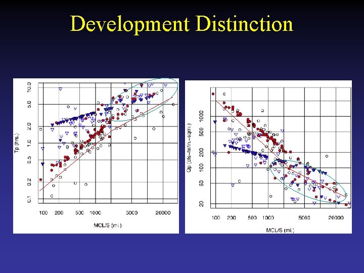
Development Distinction

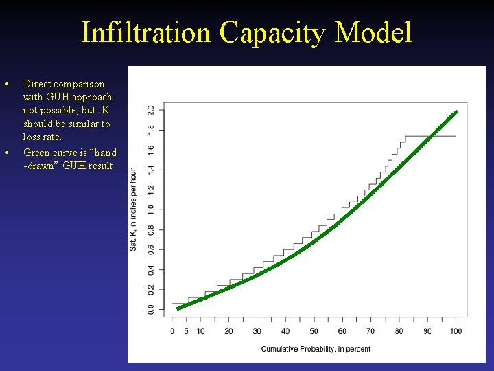
Infiltration Capacity Model • • Direct comparison with GUH approach not possible, but: K should be similar to loss rate. Green curve is “hand -drawn” GUH result

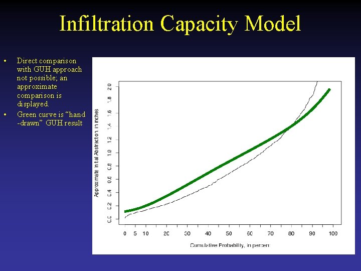
Infiltration Capacity Model • • Direct comparison with GUH approach not possible; an approximate comparison is displayed. Green curve is “hand -drawn” GUH result

Summary • Based on all approaches: – Urbanization cuts time to peak in half, which substantially increases peak discharge. – Unit hydrographs can be reliably estimated for many watersheds based on physical characteristics. – Understand time and one understands the hydrograph. – Dimensionless hydrograph shapes for developed and undeveloped watersheds are similar.

Summary • Based on Gamma approach: – Constant loss (0. 5 in/hr) – Initial abstraction is about 1. 1 in. (undeveloped) and 0. 5 in. (developed). – Urbanization cuts initial abstraction by about half. – Urbanization apparently has limited influence on constant loss for macrowatersheds?

Summary • Based on GIUH approach: – Asymptotic loss (0. 8 in/hr) (Comparable). – Initial abstraction approximation is 0. 6 inches (Smaller but comparable). – Urbanization distinction is expected to be comparable.

Summary • Common rainfall-runoff database. • Common concept of temporal redistribution of excess rainfall. • Otherwise independent procedures produce comparable results! • For appropriate watersheds: – GUH tool is developed. – GIUH is a research tool to explore ensemble approaches.

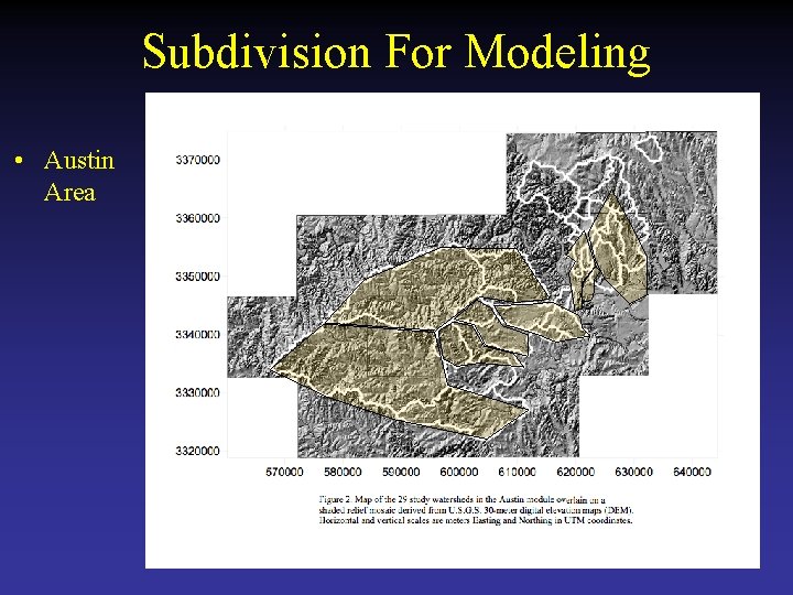
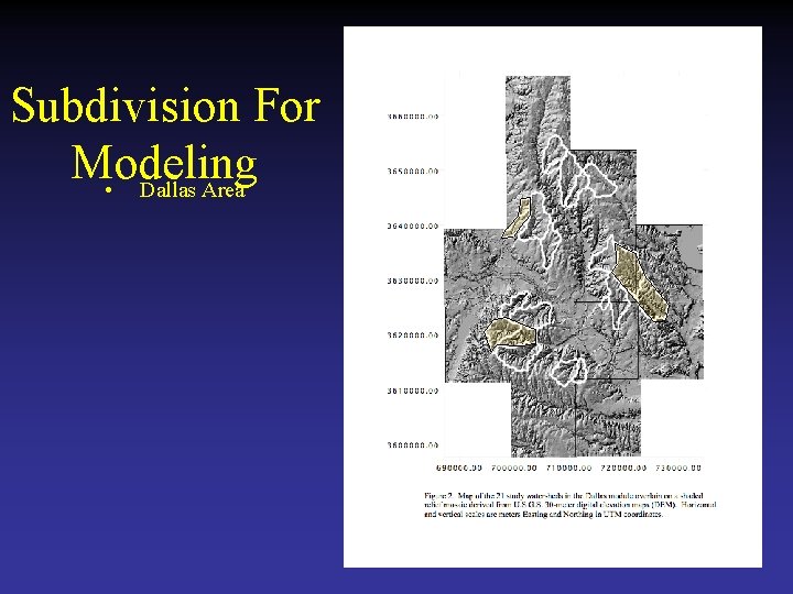
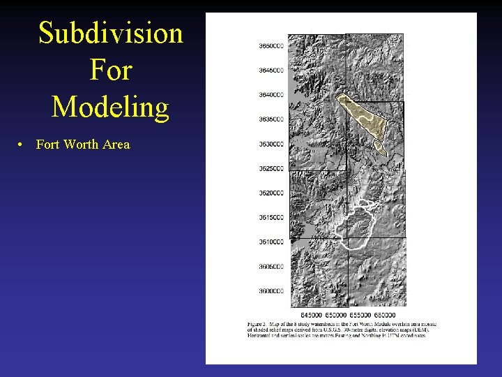
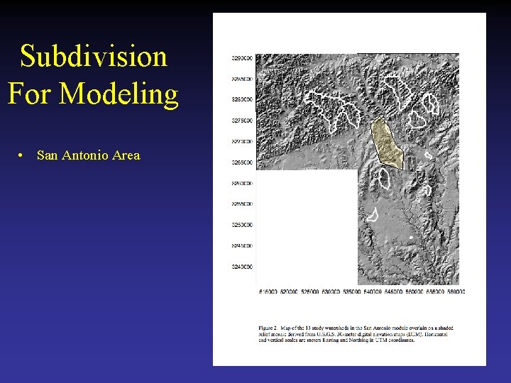
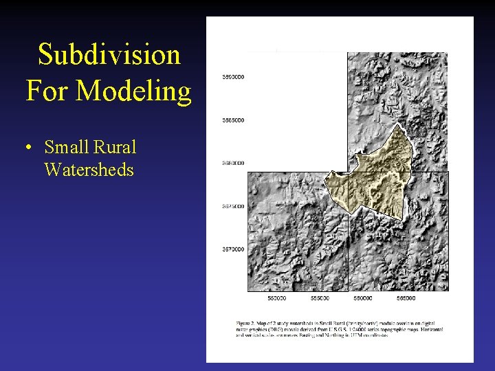
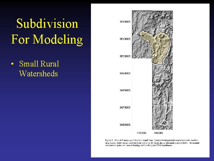
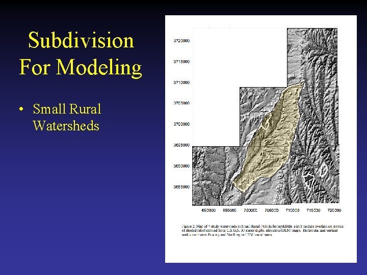
Subdivision For Modeling • From the existing database – 17 Superset watersheds with gaged subset sub-areas. • • • 8 Austin 3 Dallas 2 Fort Worth 1 San Antonio 3 Small Rural Watersheds – 15 Supersets have paired rainfall-runoff events for all sub-areas.

Subdivision For Modeling • Austin Area

Subdivision For Modeling • Dallas Area

Subdivision For Modeling • Fort Worth Area

Subdivision For Modeling • San Antonio Area

Subdivision For Modeling • Small Rural Watersheds

Subdivision For Modeling • Small Rural Watersheds

Subdivision For Modeling • Small Rural Watersheds

Subdivision For Modeling • These watersheds represent a set of test cases for subdivision testing. – Some are divided roughly equal area. – Some have vastly different sub-areas. • These differences are serendipitous because they allow some testing of schemes suggested by literature

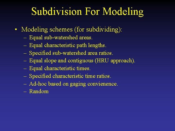
Subdivision For Modeling • Modeling schemes (for subdividing): – – – – Equal sub-watershed areas. Equal characteristic path lengths. Specified sub-watershed area ratios. Equal slope and contiguous (HRU approach). Equal characteristic times. Specified characteristic time ratios. Ad-hoc based on gaging convienence. Random

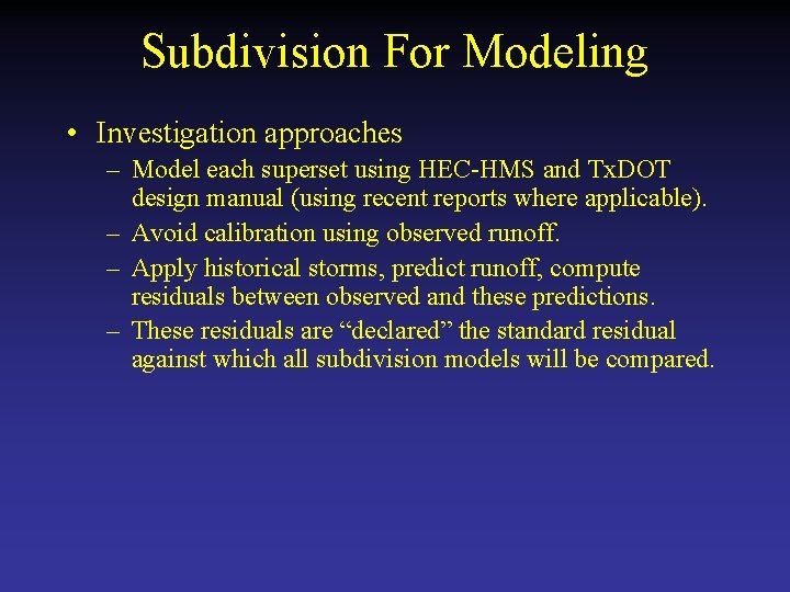
Subdivision For Modeling • Investigation approaches – Model each superset using HEC-HMS and Tx. DOT design manual (using recent reports where applicable). – Avoid calibration using observed runoff. – Apply historical storms, predict runoff, compute residuals between observed and these predictions. – These residuals are “declared” the standard residual against which all subdivision models will be compared.

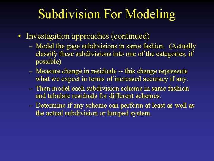
Subdivision For Modeling • Investigation approaches (continued) – Model the gage subdivisions in same fashion. (Actually classify these subdivisions into one of the categories, if possible) – Measure change in residuals -- this change represents what we expect in terms of increased accuracy if any. – Then model each subdivision scheme in same fashion and tabulate residuals for different schemes. – Determine if any scheme can perform at least as well as the actual subdivision or lumped system.

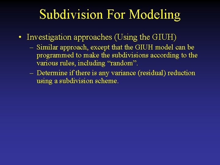
Subdivision For Modeling • Investigation approaches (Using the GIUH) – Similar approach, except that the GIUH model can be programmed to make the subdivisions according to the various rules, including “random”. – Determine if there is any variance (residual) reduction using a subdivision scheme.

Publications: • http: //library. ctr. utexas. edu/dbtwwpd/textbase/websearchcat. htm (Search for authors: Asquith; Roussel; Thompson; Fang; or Cleveland). • http: //cleveland 1. cive. uh. edu/publications (selected papers on-line). • http: //infotrek. er. usgs. gov/pubs/ (Search for author Asquith; Roussel) • http: //www. techmrt. ttu. edu/reports. php (Search for author Thompson) • http: //ceserver. lamar. edu/People/fang/research. html