Randomized Algorithms Lecturer Moni Naor Lecture 12 Recap

Randomized Algorithms Lecturer: Moni Naor Lecture 12

Recap and Today Recap • Cuckooh Hashing Today • Cuckoo Hashing • Bloom Filters • Random Graphs • Limited Randomness and the Braverman’s Result concerning AC 0

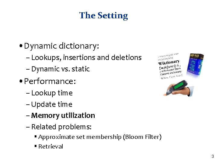
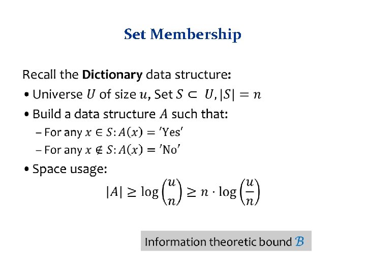
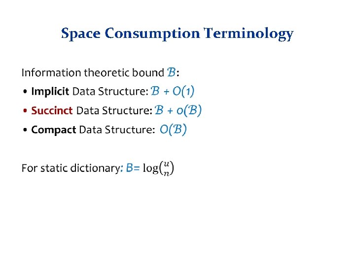
The Setting • Dynamic dictionary: – Lookups, insertions and deletions – Dynamic vs. static • Performance: – Lookup time – Update time – Memory utilization – Related problems: § Approximate set membership (Bloom Filter) § Retrieval 3

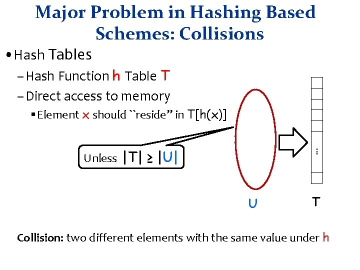
Major Problem in Hashing Based Schemes: Collisions • Hash Tables – Hash Function h Table T – Direct access to memory § Element x should ``reside” in T[h(x)]. . . Unless |T| ≥ |U| U T Collision: two different elements with the same value under h

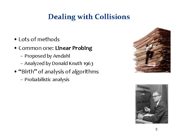
Dealing with Collisions • Lots of methods • Common one: Linear Probing – Proposed by Amdahl – Analyzed by Donald Knuth 1963 • “Birth” of analysis of algorithms – Probabilistic analysis 5

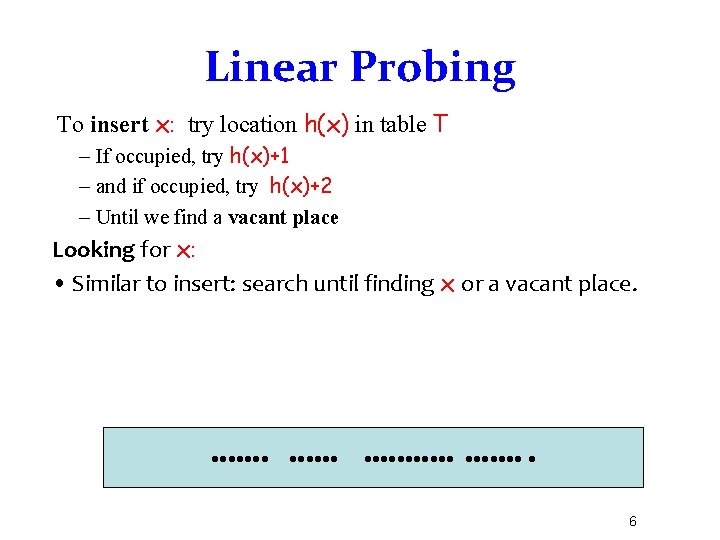
Linear Probing To insert x: try location h(x) in table T – If occupied, try h(x)+1 – and if occupied, try h(x)+2 – Until we find a vacant place Looking for x: • Similar to insert: search until finding x or a vacant place. 6

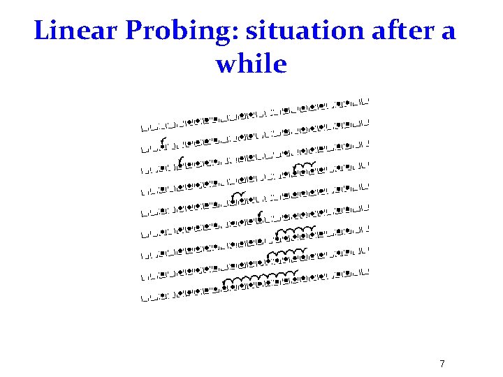
Linear Probing: situation after a while 7

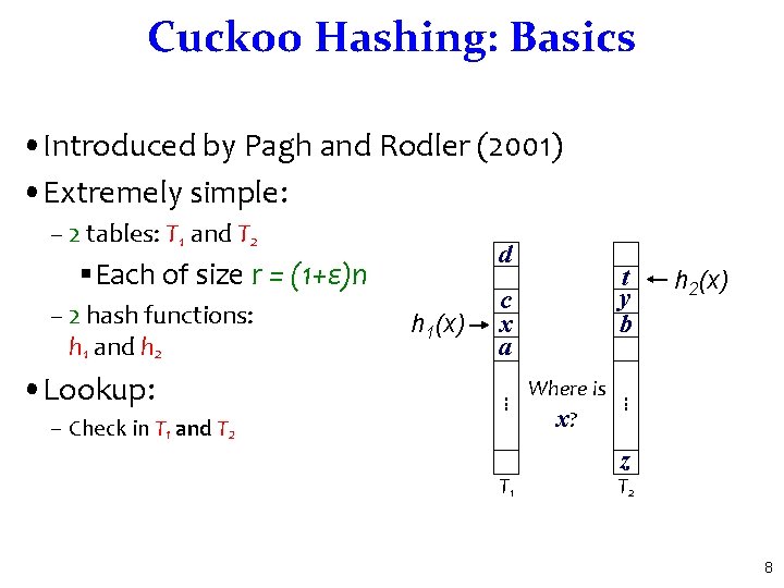
Cuckoo Hashing: Basics • Introduced by Pagh and Rodler (2001) • Extremely simple: – 2 tables: T 1 and T 2 d §Each of size r = (1+ε)n – 2 hash functions: h 1 and h 2 c x a – Check in T 1 and T 2 T 1 Where is x? h 2(x) . . . • Lookup: h 1(x) t y b z T 2 8

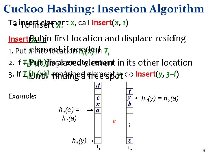
Cuckoo Hashing: Insertion Algorithm To element • insert To insert x: x, call Insert(x, 1) – Puti): in first location and displace residing Insert(x, if needed 1. Put xelement into location hi(x) in Ti 2. If T–i[h was empty: return in its other location Put displaced element i(x)] 3. If – Ti[h y: do Insert(y, 3–i) i(x)] contained Until finding a element free spot d Example: T 1 e h 2(y) = h 2(a) . . . h 1(y) c x a. . . h 1(e) = h 1(a) t y b z T 2 9

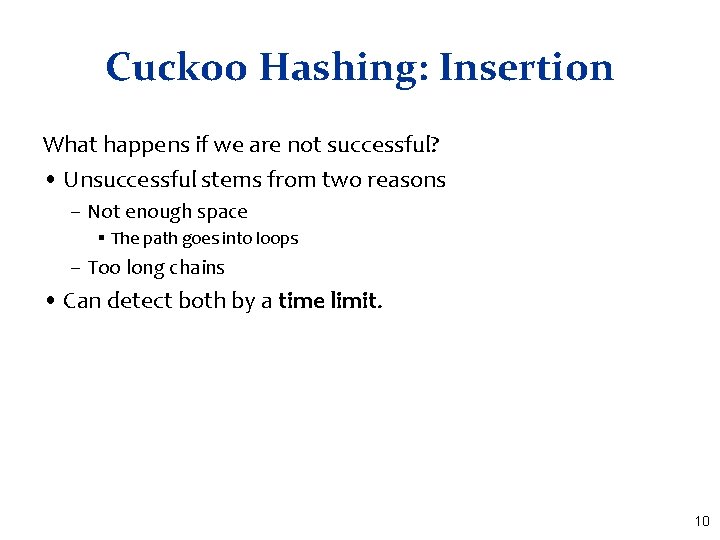
Cuckoo Hashing: Insertion What happens if we are not successful? • Unsuccessful stems from two reasons – Not enough space § The path goes into loops – Too long chains • Can detect both by a time limit. 10

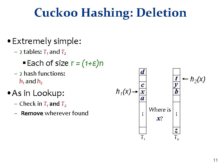
Cuckoo Hashing: Deletion • Extremely simple: – 2 tables: T 1 and T 2 §Each of size r = (1+ε)n d – 2 hash functions: h 1 and h 2 • As in Lookup: c x a T 1 Where is x? h 2(x) . . . – Check in T 1 and T 2 – Remove wherever found h 1(x) t y b z T 2 11

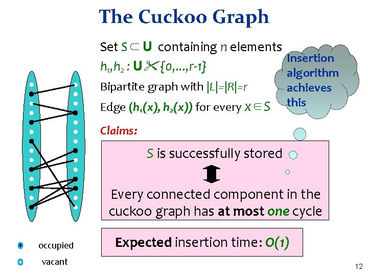
The Cuckoo Graph Set S ⊂ U containing n elements Insertion h 1, h 2 : U {0, . . . , r-1} algorithm Bipartite graph with |L|=|R|=r Edge (h 1(x), h 2(x)) for every x∈S achieves this Claims: S is successfully stored Every connected component in the cuckoo graph has at most one cycle occupied vacant Expected insertion time: O(1) 12

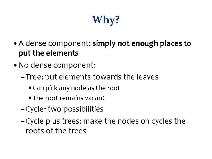
Why? • A dense component: simply not enough places to put the elements • No dense component: – Tree: put elements towards the leaves § Can pick any node as the root § The root remains vacant – Cycle: two possibilities – Cycle plus trees: make the nodes on cycles the roots of the trees

Cuckoo Hashing: Properties • Many attractive properties: – Lookup and deletion in 2 accesses in the worst case § May be done in parallel – Insertion takes amortized constant time – Reasonable memory utilization – No dynamic memory allocation • Lots of Generalizations • Lots of applications to related problems • Growing evidence of practicality on current architectures 14

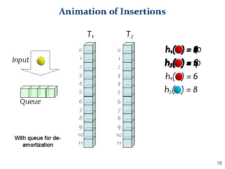
Animation of Insertions T 1 Input Queue With queue for deamortization T 2 0 1 2 3 4 5 6 7 8 9 10 11 h 11( h 22( h 1( h 2( 8 6 2 ) = 410 ) = 10 4168 )=6 )=8 15

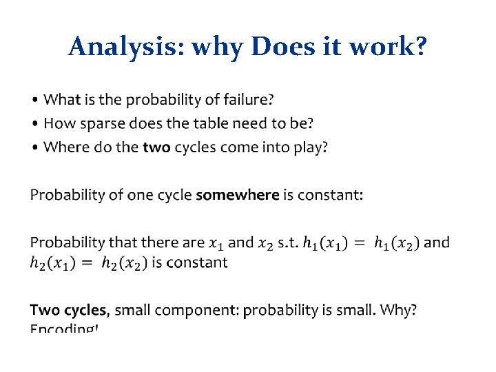
More than One Cycle • With probability Θ(1/n) Cuckoo Hashing fails – Recall: connected component with more than one cycle – Standard solution: rehashing §Meaning: insertion worst case may be O(n) • [KMW 08] suggested stash Kirsch, Mitzenmacher, – Saves rehashing Wieder §Actually reduces insertion worst case to O(log n) – Constant-sized stash is sufficient whp Prob of more than k: 1/nk+1 16

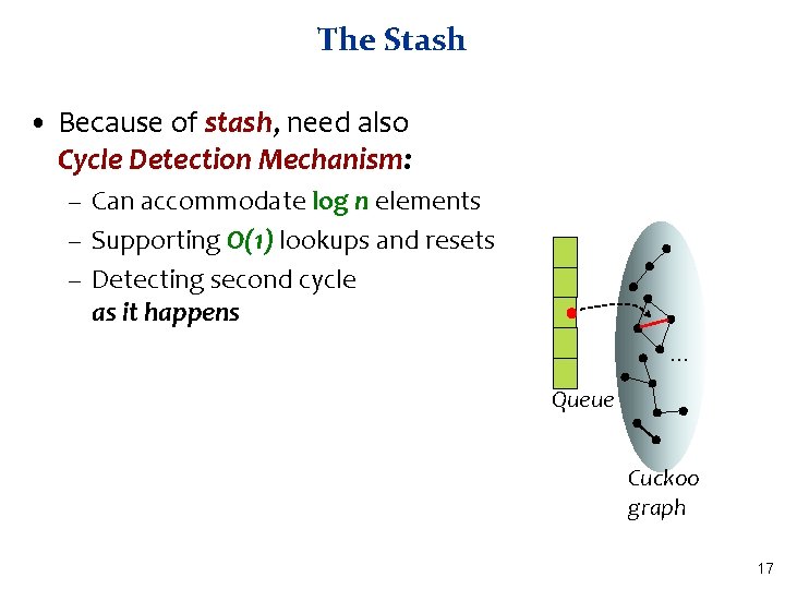
The Stash • Because of stash, need also Cycle Detection Mechanism: – Can accommodate log n elements – Supporting O(1) lookups and resets – Detecting second cycle as it happens. . . Queue Cuckoo graph 17

Analysis: why Does it work? •

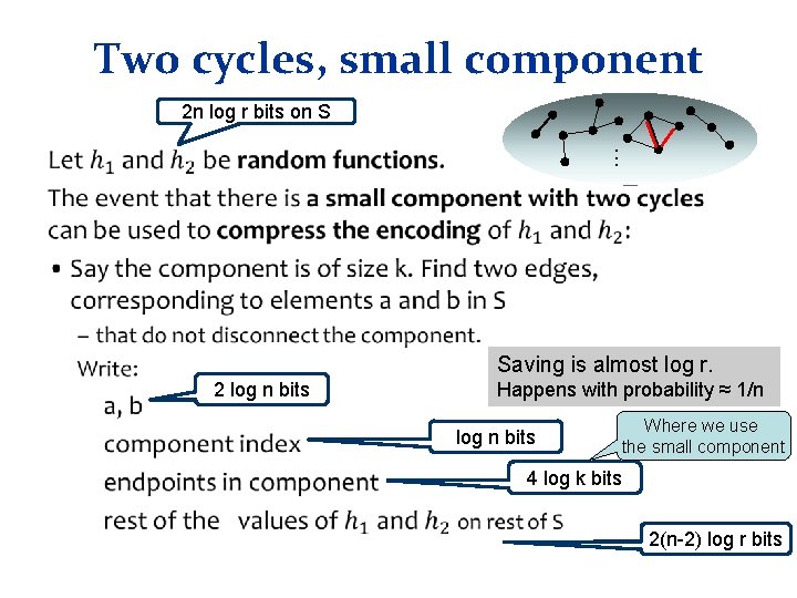
Two cycles, small component 2 n log r bits on S . . . • Saving is almost log r. 2 log n bits Happens with probability ≈ 1/n log n bits Where we use the small component 4 log k bits 2(n-2) log r bits

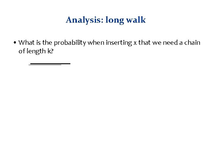
Analysis: long walk • What is the probability when inserting x that we need a chain of length k?

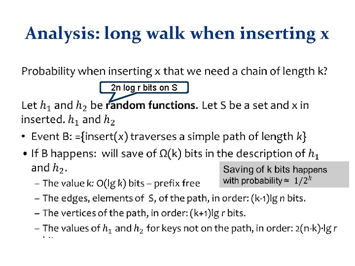
Analysis: long walk when inserting x • 2 n log r bits on S

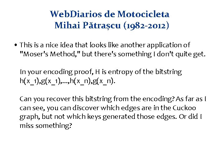
Web. Diarios de Motocicleta Mihai Pătrașcu (1982 -2012) • This is a nice idea that looks like another application of "Moser's Method, " but there's something I don't quite get. In your encoding proof, H is entropy of the bitstring h(x_1), g(x_1), . . . , h(x_n), g(x_n). Can you recover this bitstring from the encoding? As far as I can see, you can discover which edges are in the Cuckoo graph, but not which keys generated those edges. Or did I miss something?

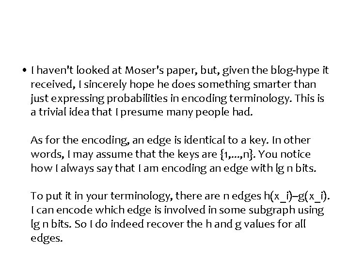
• I haven't looked at Moser's paper, but, given the blog-hype it received, I sincerely hope he does something smarter than just expressing probabilities in encoding terminology. This is a trivial idea that I presume many people had. As for the encoding, an edge is identical to a key. In other words, I may assume that the keys are {1, . . . , n}. You notice how I always say that I am encoding an edge with lg n bits. To put it in your terminology, there are n edges h(x_i)--g(x_i). I can encode which edge is involved in some subgraph using lg n bits. So I do indeed recover the h and g values for all edges.

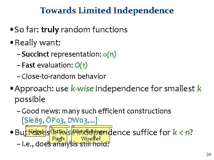
Towards Limited Independence • So far: truly random functions • Really want: – Succinct representation: o(n) – Fast evaluation: O(1) – Close-to-random behavior • Approach: use k-wise independence for smallest k possible – Good news: many such efficient constructions [Sie 89, ÖP 03, DW 03, . . . ] • But: Siegel doesÖstlin, k-wise. Dietzfelbinger, independence suffice for k < n? Pagh Woelfel – I. e. , does analysis still hold? 24

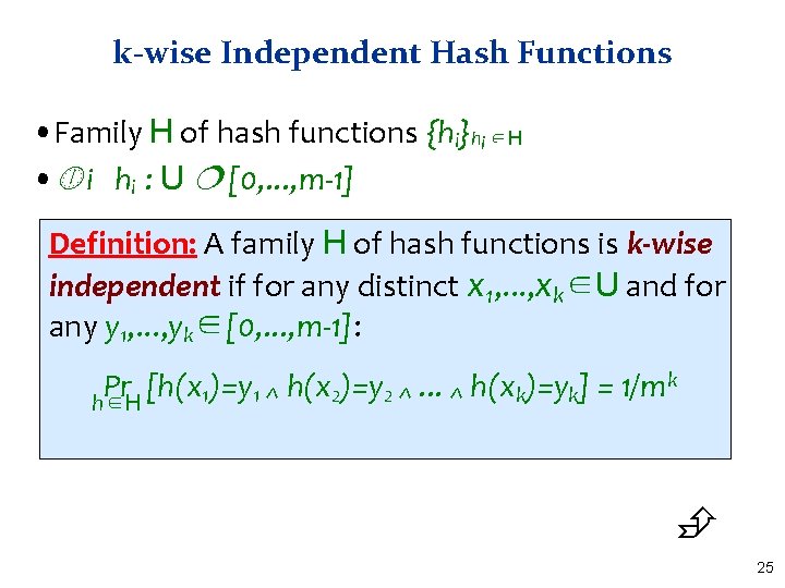
k-wise Independent Hash Functions • Family H of hash functions {hi}hi ∈H • i hi : U [0, . . . , m-1] Definition: A family H of hash functions is k-wise independent if for any distinct x 1, . . . , xk∈U and for any y 1, . . . , yk∈[0, . . . , m-1]: k Pr [h(x )=y. . . h(x )=y ] = 1/m 1 1^ 2 2^ k k ^ h∈H 25

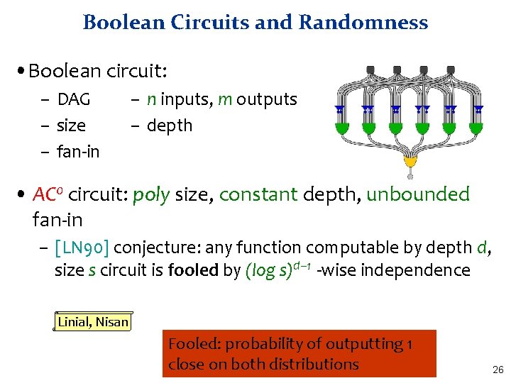
Boolean Circuits and Randomness • Boolean circuit: – DAG – size – fan-in – n inputs, m outputs – depth • AC 0 circuit: poly size, constant depth, unbounded fan-in – [LN 90] conjecture: any function computable by depth d, size s circuit is fooled by (log s)d– 1 -wise independence Linial, Nisan Fooled: probability of outputting 1 close on both distributions 26

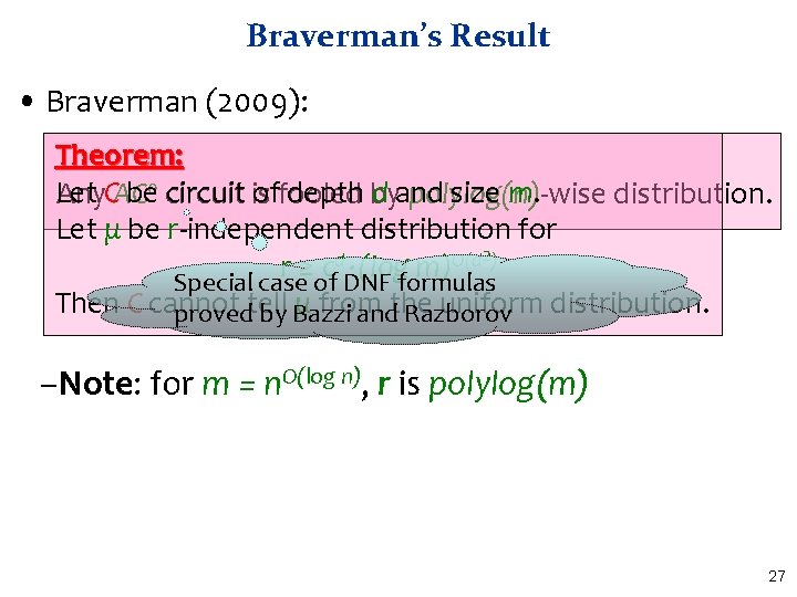
Braverman’s Result • Braverman (2009): Theorem: Let be 0 circuit is offooled depth by d and size m. Any. CAC polylog(n)-wise distribution. Let μ be r-independent distribution for 2) d O(d r ≥ c · (log m) Special case of DNF formulas Then C cannot μ from uniform distribution. provedtell by Bazzi andthe Razborov –Note: for m = n. O(log n), r is polylog(m) 27

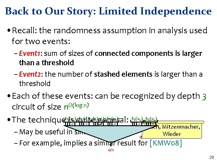
Back to Our Story: Limited Independence • Recall: the randomness assumption in analysis used for two events: – Event 1: sum of sizes of connected components is larger than a threshold – Event 2: the number of stashed elements is larger than a threshold • Each of these events: can be recognized by depth 3 circuit of size n. O(log n) (x ) h (x ) • The techniquehis quite general: h (x ) 1 1 . . . 2 1 . . . 1 2 . . . 2 2 . . . 1 k . . . 2 k . . . Kirsch, Mitzenmacher, Wieder – May be useful in similar scenarios – For example, implies a similar result for [KMW 08] 0/1 28

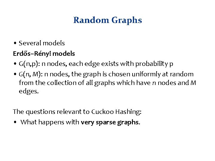
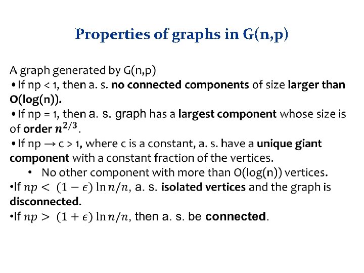
Random Graphs • Several models Erdős–Rényi models • G(n, p): n nodes, each edge exists with probability p • G(n, M): n nodes, the graph is chosen uniformly at random from the collection of all graphs which have n nodes and M edges. The questions relevant to Cuckoo Hashing: • What happens with very sparse graphs.

Properties of graphs in G(n, p)

Set Membership •

Space Consumption Terminology •

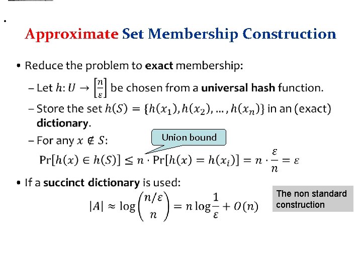
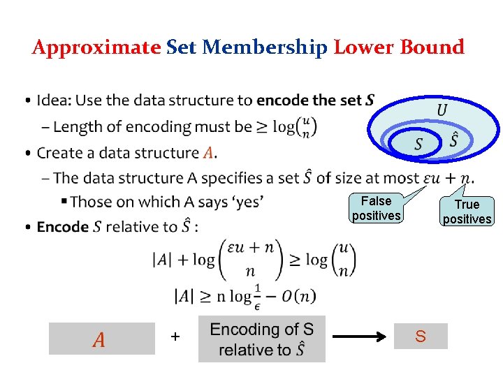
Approximate Set Membership •

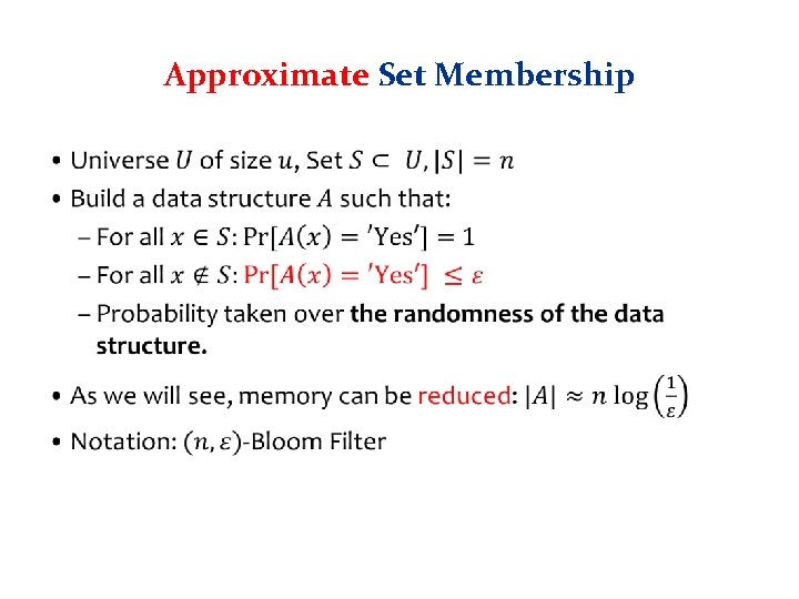
• Approximate Set Membership Construction • Union bound The non standard construction

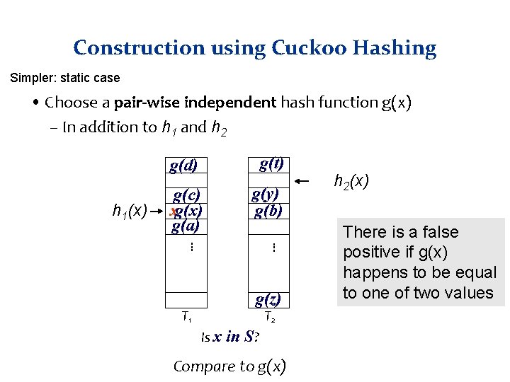
Construction using Cuckoo Hashing Simpler: static case • Choose a pair-wise independent hash function g(x) – In addition to h 1 and h 2 h 1(x) g(d) g(t) g(c) xg(x) g(a) g(y) g(b). . . g(z) T 2 T 1 Is x in S? Compare to g(x) h 2(x) There is a false positive if g(x) happens to be equal to one of two values

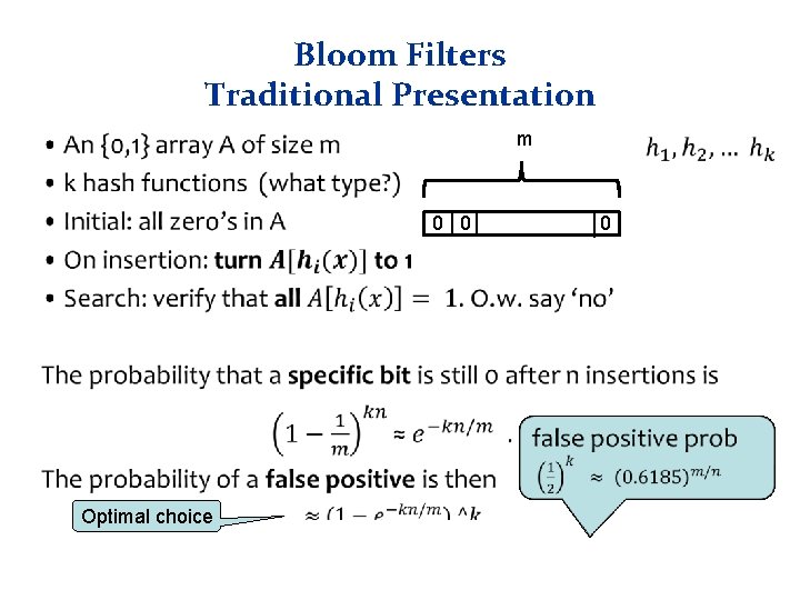
Bloom Filters Traditional Presentation • m 0 0 Optimal choice 0

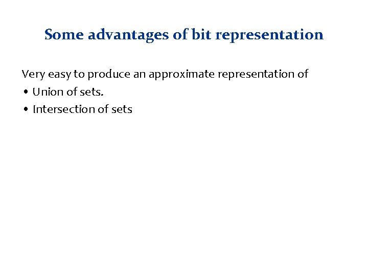
Some advantages of bit representation Very easy to produce an approximate representation of • Union of sets. • Intersection of sets

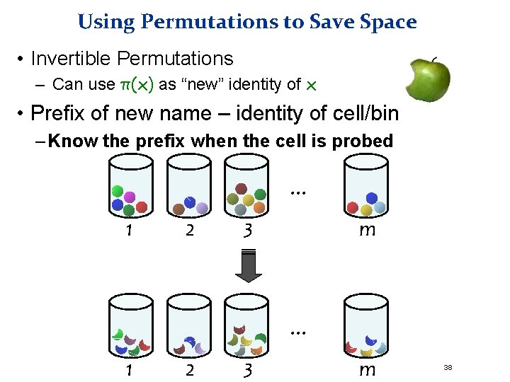
Using Permutations to Save Space • Invertible Permutations – Can use π(x) as “new” identity of x • Prefix of new name – identity of cell/bin – Know the prefix when the cell is probed . . . 1 2 m 3 . . . 1 2 3 m 38

Approximate Set Membership Lower Bound • False positives + True positives S

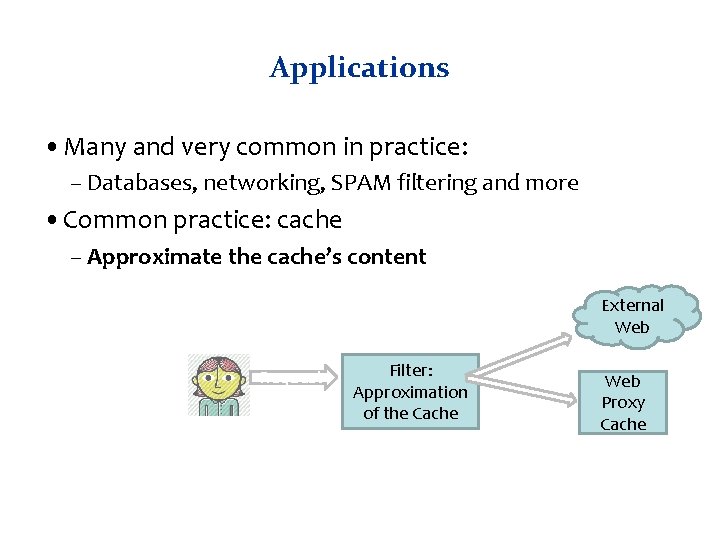
Applications • Many and very common in practice: – Databases, networking, SPAM filtering and more • Common practice: cache – Approximate the cache’s content External Web Request Filter: Approximation of the Cache Web Proxy Cache

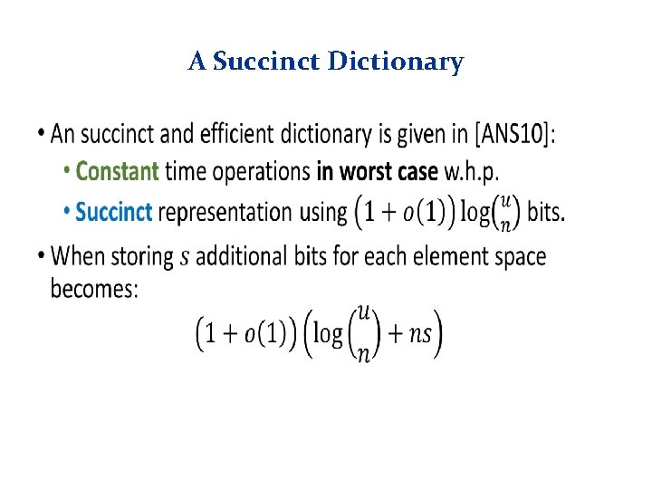
A Succinct Dictionary •