Complexity Theory Lecture 11 Lecturer Moni Naor Recap

Complexity Theory Lecture 11 Lecturer: Moni Naor

Recap Last week: Statistical zero-knowledge AM protocol for VC dimension Hardness and Randomness This Week: Hardness and Randomness Semi-Random Sources Extractors

Derandomization A major research question: • How to make the construction of – Small Sample space `resembling’ large one – Hitting sets Efficient. Successful approach: randomness from hardness – (Cryptographic) pseudo-random generators – Complexity oriented pseudo-random generators

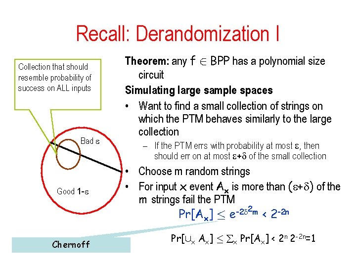
Recall: Derandomization I Collection that should resemble probability of success on ALL inputs Bad Good 1 - Chernoff Theorem: any f 2 BPP has a polynomial size circuit Simulating large sample spaces • Want to find a small collection of strings on which the PTM behaves similarly to the large collection – If the PTM errs with probability at most , then should err on at most + of the small collection • Choose m random strings • For input x event Ax is more than ( + ) of the m strings fail the PTM 2 m -2 Pr[Ax] · e < 2 -2 n Pr[[x Ax] · x Pr[Ax] < 2 n 2 -2 n=1

Pseudo-random generators • Would like to stretch a short secret (seed) into a long one • The resulting long string should be usable in any case where a long string is needed – In particular: cryptographic application as a one-time pad • Important notion: Indistinguishability Two probability distributions that cannot be distinguished – Statistical indistinguishability: distances between probability distributions – New notion: computational indistinguishability

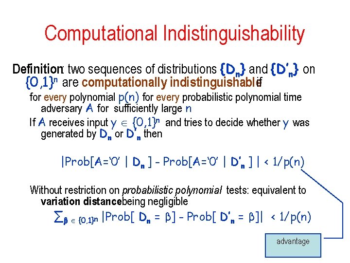
Computational Indistinguishability Definition: two sequences of distributions {Dn} and {D’n} on {0, 1}n are computationally indistinguishableif for every polynomial p(n) for every probabilistic polynomial time adversary A for sufficiently large n If A receives input y {0, 1}n and tries to decide whether y was generated by Dn or D’n then |Prob[A=‘ 0’ | Dn ] - Prob[A=‘ 0’ | D’n ] | < 1/p(n) Without restriction on probabilistic polynomial tests: equivalent to variation distancebeing negligible ∑β {0, 1}n |Prob[ Dn = β] - Prob[ D’n = β]| < 1/p(n) advantage

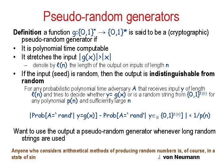
Pseudo-random generators Definition: a function g: {0, 1}* → {0, 1}* is said to be a (cryptographic) pseudo-random generator if • It is polynomial time computable • It stretches the input |g(x)|>|x| – denote by ℓ(n) the length of the output on inputs of length n • If the input (seed) is random, then the output is indistinguishable from random For any probabilistic polynomial time adversary A that receives input y of length ℓ(n) and tries to decide whether y= g(x) or is a random string from {0, 1}ℓ(n) for any polynomial p(n) and sufficiently large n |Prob[A=`rand’| y=g(x)] - Prob[A=`rand’| y R {0, 1}ℓ(n)] | < 1/p(n) Want to use the output a pseudo-random generator whenever long random strings are used Anyone who considers arithmetical methods of producing random numbers is, of course, in a state of sin. J. von Neumann

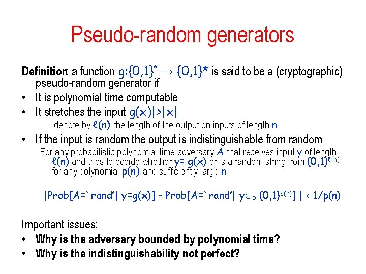
Pseudo-random generators Definition: a function g: {0, 1}* → {0, 1}* is said to be a (cryptographic) pseudo-random generator if • It is polynomial time computable • It stretches the input g(x)|>|x| – denote by ℓ(n) the length of the output on inputs of length n • If the input is random the output is indistinguishable from random For any probabilistic polynomial time adversary A that receives input y of length ℓ(n) and tries to decide whether y= g(x) or is a random string from {0, 1}ℓ(n) for any polynomial p(n) and sufficiently large n |Prob[A=`rand’| y=g(x)] - Prob[A=`rand’| y R {0, 1}ℓ(n)] | < 1/p(n) Important issues: • Why is the adversary bounded by polynomial time? • Why is the indistinguishability not perfect?

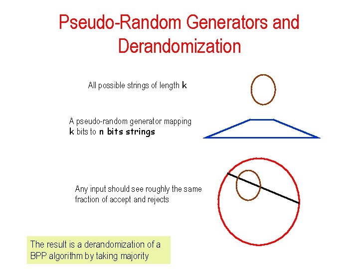
Pseudo-Random Generators and Derandomization All possible strings of length k A pseudo-random generator mapping k bits to n bits strings Any input should see roughly the same fraction of accept and rejects The result is a derandomization of a BPP algorithm by taking majority

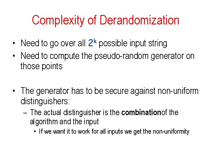
Complexity of Derandomization • Need to go over all 2 k possible input string • Need to compute the pseudo-random generator on those points • The generator has to be secure against non-uniform distinguishers: – The actual distinguisher is the combinationof the algorithm and the input • If we want it to work for all inputs we get the non-uniformity

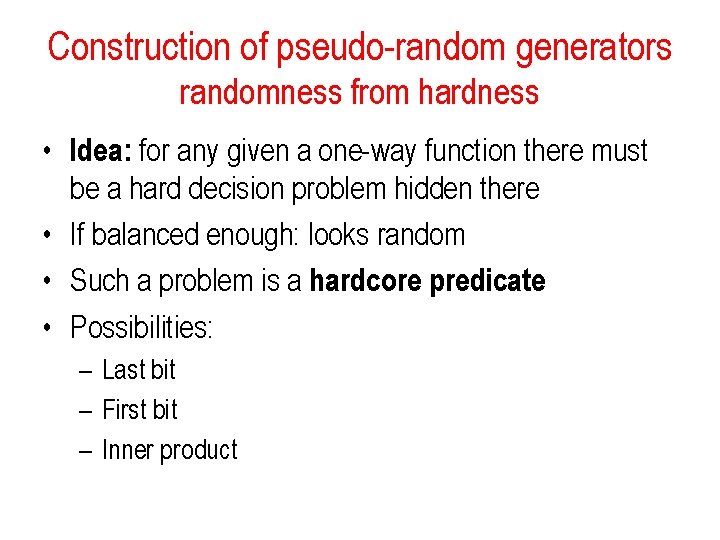
Construction of pseudo-random generators randomness from hardness • Idea: for any given a one-way function there must be a hard decision problem hidden there • If balanced enough: looks random • Such a problem is a hardcore predicate • Possibilities: – Last bit – First bit – Inner product

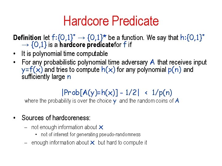
Hardcore Predicate Definition: let f: {0, 1}* → {0, 1}* be a function. We say that h: {0, 1}* → {0, 1} is a hardcore predicate for f if • It is polynomial time computable • For any probabilistic polynomial time adversary A that receives input y=f(x) and tries to compute h(x) for any polynomial p(n) and sufficiently large n |Prob[A(y)=h(x)] - 1/2| < 1/p(n) where the probability is over the choice y and the random coins of A • Sources of hardcoreness: – not enough information about x • not of interest for generating pseudo-randomness – enough information about x but hard to compute it

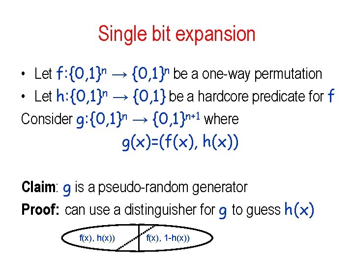
Single bit expansion • Let f: {0, 1}n → {0, 1}n be a one-way permutation • Let h: {0, 1}n → {0, 1} be a hardcore predicate for f Consider g: {0, 1}n → {0, 1}n+1 where g(x)=(f(x), h(x)) Claim: g is a pseudo-random generator Proof: can use a distinguisher for g to guess h(x) f(x), h(x)) f(x), 1 -h(x))

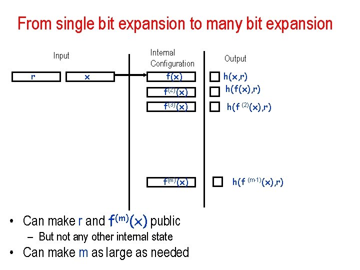
From single bit expansion to many bit expansion Input r x Internal Configuration f(x) f(2)(x) f(3)(x) f(m)(x) • Can make r and f(m)(x) public – But not any other internal state • Can make m as large as needed Output h(x, r) h(f(x), r) h(f (2)(x), r) h(f (m-1)(x), r)

Two important techniques for showing pseudo-randomness • Hybrid argument • Next-bit prediction and pseudo-randomness

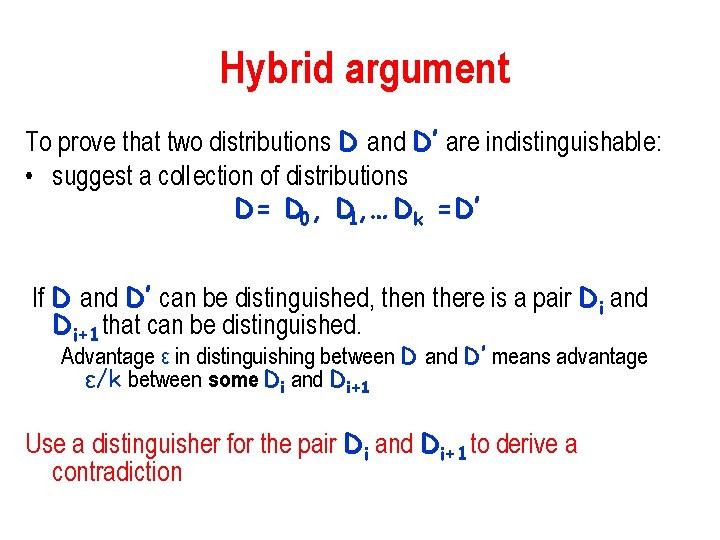
Hybrid argument To prove that two distributions D and D’ are indistinguishable: • suggest a collection of distributions D= D 0, D 1, … Dk =D’ If D and D’ can be distinguished, then there is a pair Di and Di+1 that can be distinguished. Advantage ε in distinguishing between D and D’ means advantage ε/k between some Di and Di+1 Use a distinguisher for the pair Di and Di+1 to derive a contradiction

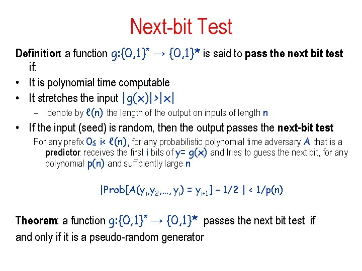
Next-bit Test Definition: a function g: {0, 1}* → {0, 1}* is said to pass the next bit test if: • It is polynomial time computable • It stretches the input |g(x)|>|x| – denote by ℓ(n) the length of the output on inputs of length n • If the input (seed) is random, then the output passes the next-bit test For any prefix 0≤ i< ℓ(n), for any probabilistic polynomial time adversary A that is a predictor: receives the first i bits of y= g(x) and tries to guess the next bit, for any polynomial p(n) and sufficiently large n |Prob[A(yi, y 2, …, yi) = yi+1] – 1/2 | < 1/p(n) Theorem: a function g: {0, 1}* → {0, 1}* passes the next bit test if and only if it is a pseudo-random generator

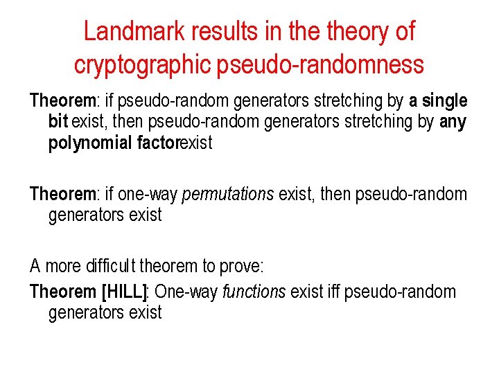
Landmark results in theory of cryptographic pseudo-randomness Theorem: if pseudo-random generators stretching by a single bit exist, then pseudo-random generators stretching by any polynomial factorexist Theorem: if one-way permutations exist, then pseudo-random generators exist A more difficult theorem to prove: Theorem [HILL]: One-way functions exist iff pseudo-random generators exist

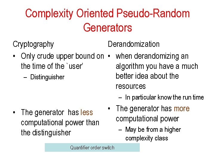
Complexity Oriented Pseudo-Random Generators Cryptography Derandomization • Only crude upper bound on • when derandomizing an the time of the `user’ algorithm you have a much better idea about the – Distinguisher resources – In particular know the run time • The generator has more • The generator has less computational power than – May be from a higher the distinguisher complexity class Quantifier order switch

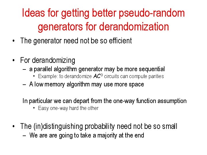
Ideas for getting better pseudo-random generators for derandomization • The generator need not be so efficient • For derandomizing – a parallel algorithm generator may be more sequential • Example: to derandomize AC 0 circuits can compute parities – A low memory algorithm may use more space In particular we can depart from the one-way function assumption • Easy one-way hard the other • The (in)distinguishing probability need not be so small – We are going to take a majority at the end

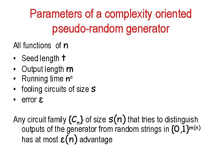
Parameters of a complexity oriented pseudo-random generator All functions of n • • • Seed length t Output length m Running time nc fooling circuits of size s error ε Any circuit family {Cn} of size s(n) that tries to distinguish outputs of the generator from random strings in {0, 1}m(n) has at most ε(n) advantage

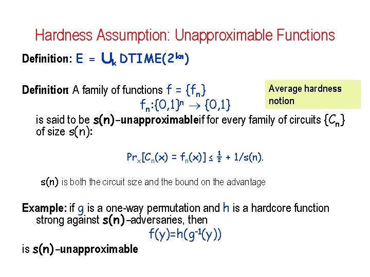
Hardness Assumption: Unapproximable Functions Definition: E = [k DTIME(2 kn) Average hardness Definition: A family of functions f = {fn} notion fn: {0, 1}n {0, 1} is said to be s(n)-unapproximableif for every family of circuits {Cn} of size s(n): Prx[Cn(x) = fn(x)] ≤ ½ + 1/s(n) is both the circuit size and the bound on the advantage Example: if g is a one-way permutation and h is a hardcore function strong against s(n)-adversaries, then f(y)=h(g-1(y)) is s(n)-unapproximable

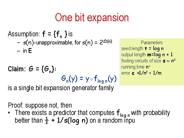
One bit expansion Assumption: f = {fn } is – s(n)-unapproximable, for s(n) = 2Ω(n) – in E Claim: G = {Gn}: Gn(y) = y◦flog n(y) is a single bit expansion generator family Parameters seed length t = log n output length m=log n + 1 fooling circuits of size s nδ running time nc error ε =1/nδ < 1/m Proof: suppose not, then • There exists a predictor that computes flog n with probability better than ½ + 1/s(log n) on a random inpu

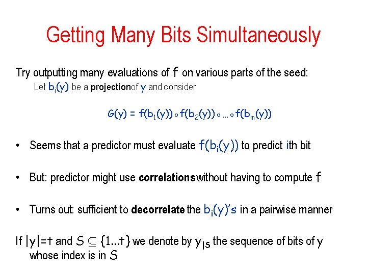
Getting Many Bits Simultaneously Try outputting many evaluations of f on various parts of the seed: Let bi(y) be a projectionof y and consider G(y) = f(b 1(y))◦f(b 2(y))◦…◦f(bm(y)) • Seems that a predictor must evaluate f(bi(y)) to predict ith bit • But: predictor might use correlationswithout having to compute f • Turns out: sufficient to decorrelate the bi(y)’s in a pairwise manner If |y|=t and S µ {1. . . t} we denote by y|S the sequence of bits of y whose index is in S

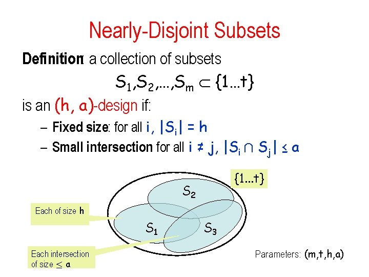
Nearly-Disjoint Subsets Definition: a collection of subsets S 1, S 2, …, Sm {1…t} is an (h, a)-design if: – Fixed size: for all i, |Si| = h – Small intersection: for all i ≠ j, |Si Å Sj| ≤ a {1. . . t} S 2 Each of size h S 1 Each intersection of size · a S 3 Parameters: (m, t, h, a)

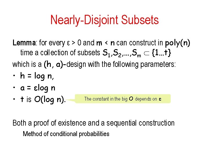
Nearly-Disjoint Subsets Lemma: for every ε > 0 and m < n can construct in poly(n) time a collection of subsets S 1, S 2, …, Sm {1…t} which is a (h, a)-design with the following parameters: • h = log n, • a = εlog n The constant in the big O depends on ε • t is O(log n). Both a proof of existence and a sequential construction Method of conditional probabilities

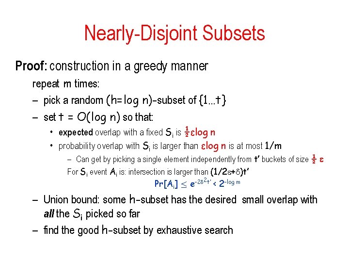
Nearly-Disjoint Subsets Proof: construction in a greedy manner repeat m times: – pick a random (h=log n)-subset of {1…t} – set t = O(log n) so that: • expected overlap with a fixed Si is ½εlog n • probability overlap with Si is larger than εlog n is at most 1/m – Can get by picking a single element independently from t’ buckets of size ½ ε For Si event Ai is: intersection is larger than (1/2 + )t’ 2 Pr[Ai] · e-2 t’ < 2 -log m – Union bound: some h-subset has the desired small overlap with all the Si picked so far – find the good h-subset by exhaustive search

Other construction of designs • Based on error correcting codes • Simple construction: based on polynomials

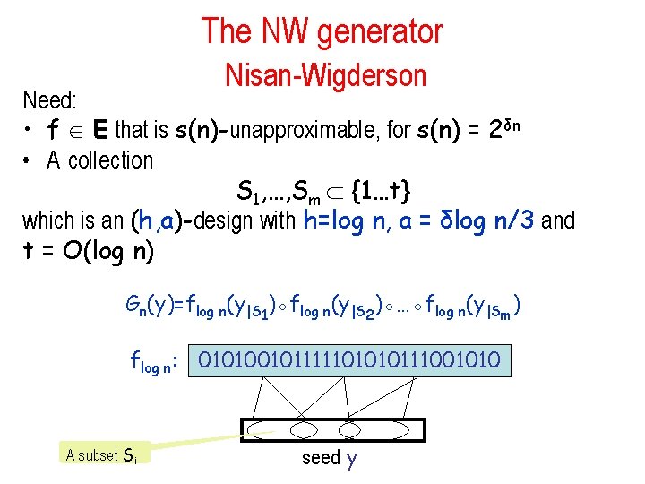
The NW generator Nisan-Wigderson Need: • f E that is s(n)-unapproximable, for s(n) = 2δn • A collection S 1, …, Sm {1…t} which is an (h, a)-design with h=log n, a = δlog n/3 and t = O(log n) Gn(y)=flog n(y|S 1)◦flog n(y|S 2)◦…◦flog n(y|Sm) flog n: 010100101111101010111001010 A subset Si seed y

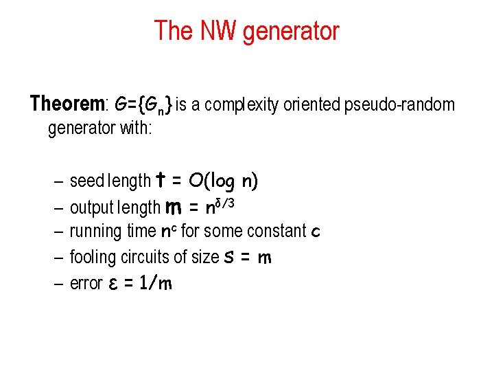
The NW generator Theorem: G={Gn} is a complexity oriented pseudo-random generator with: – – – seed length t = O(log n) output length m = nδ/3 running time nc for some constant c fooling circuits of size s = m error ε = 1/m

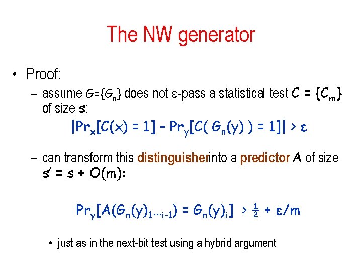
The NW generator • Proof: – assume G={Gn} does not -pass a statistical test C = {Cm} of size s: |Prx[C(x) = 1] – Pry[C( Gn(y) ) = 1]| > ε – can transform this distinguisherinto a predictor A of size s’ = s + O(m): Pry[A(Gn(y)1…i-1) = Gn(y)i] > ½ + ε/m • just as in the next-bit test using a hybrid argument

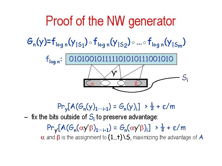
Proof of the NW generator Gn(y)=flog n(y|S 1)◦flog n(y|S 2)◦…◦flog n(y|Sm) flog n: 010100101111101010111001010 Y’ Si Pry[A(Gn(y)1…i-1) = Gn(y)i] > ½ + ε/m – fix the bits outside of Si to preserve advantage: Pry’[A(Gn( y’ )1…i-1) = Gn( y’ )i] > ½ + ε/m and is the assignment to {1…t}Si maximizing the advantage of A

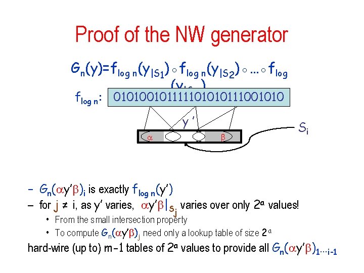
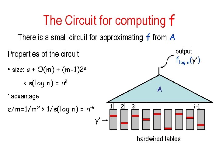
Proof of the NW generator Gn(y)=flog n(y|S 1)◦flog n(y|S 2)◦…◦flog n(y|Sm) flog n: 010100101111101010111001010 y’ Si – Gn( y’ )i is exactly flog n(y’) – for j ≠ i, as y’ varies, y’ |Sj varies over only 2 a values! • From the small intersection property • To compute Gn( y’ )j need only a lookup table of size 2 a hard-wire (up to) m-1 tables of 2 a values to provide all Gn( y’ )1…i-1

The Circuit for computing f There is a small circuit for approximating f from A output flog n(y’) Properties of the circuit • size: s + O(m) + (m-1)2 a < s(log n) = nδ A • advantage 1 ε/m=1/m 2 > 1/s(log n) = n-δ 2 3 i-1 y’ hardwired tables

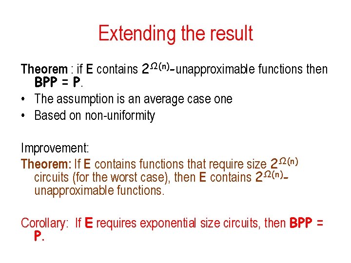
Extending the result Theorem : if E contains 2Ω(n)-unapproximable functions then BPP = P. • The assumption is an average case one • Based on non-uniformity Improvement: Theorem: If E contains functions that require size 2Ω(n) circuits (for the worst case), then E contains 2Ω(n)unapproximable functions. Corollary: If E requires exponential size circuits, then BPP = P.

Extracting Randomness from defective sources • Suppose that we have an imperfect source of randomness – physical source • biased, correlated – Collection of events in a computer • /dev/rand Information Leak • Can we: – Extract good random bits from the source – Use the source for various tasks requiring randomness • Probabilistic algorithms

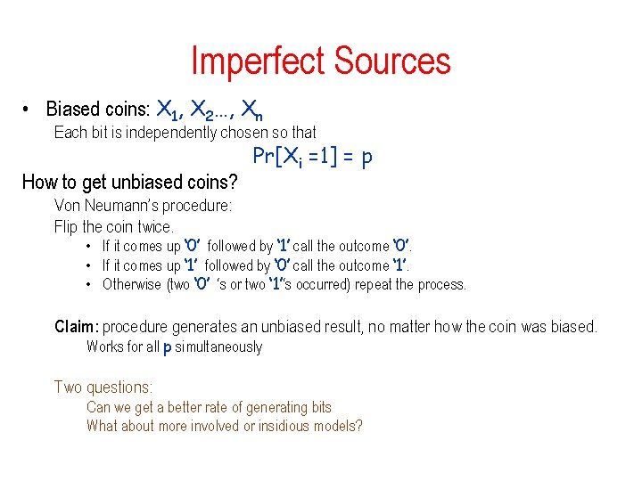
Imperfect Sources • Biased coins: X 1, X 2…, Xn Each bit is independently chosen so that How to get unbiased coins? Pr[Xi =1] = p Von Neumann’s procedure: Flip the coin twice. • If it comes up ‘ 0’ followed by ‘ 1’ call the outcome ‘ 0’. • If it comes up ‘ 1’ followed by ‘ 0’ call the outcome ‘ 1’. • Otherwise (two ‘ 0’ ‘s or two ‘ 1’‘s occurred) repeat the process. Claim: procedure generates an unbiased result, no matter how the coin was biased. Works for all p simultaneously Two questions: Can we get a better rate of generating bits What about more involved or insidious models?

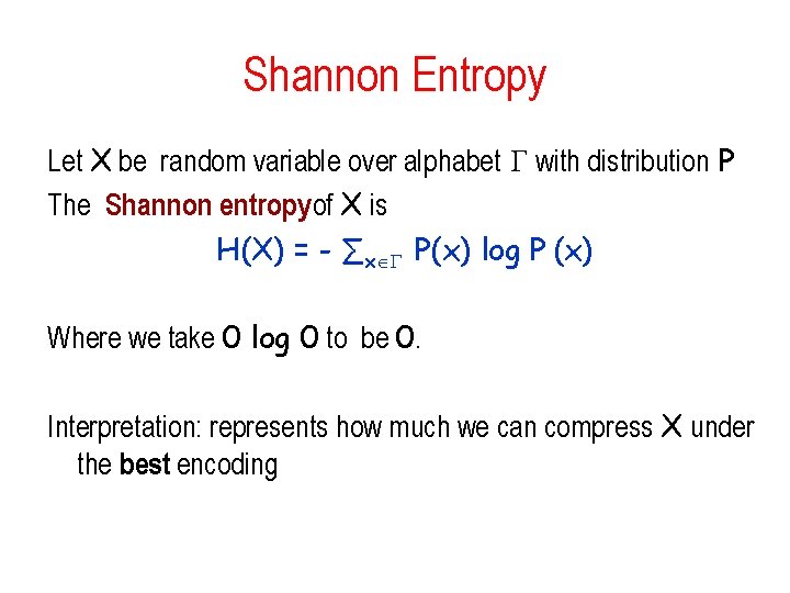
Shannon Entropy Let X be random variable over alphabet with distribution P The Shannon entropyof X is H(X) = - ∑x P(x) log P (x) Where we take 0 log 0 to be 0. Interpretation: represents how much we can compress X under the best encoding

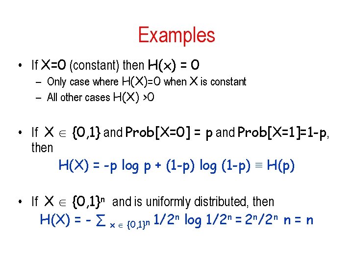
Examples • If X=0 (constant) then H(x) = 0 – Only case where H(X)=0 when X is constant – All other cases H(X) >0 • If X {0, 1} and Prob[X=0] = p and Prob[X=1]=1 -p, then H(X) = -p log p + (1 -p) log (1 -p) ≡ H(p) • If X {0, 1}n and is uniformly distributed, then H(X) = - ∑ x {0, 1}n 1/2 n log 1/2 n = 2 n/2 n n = n

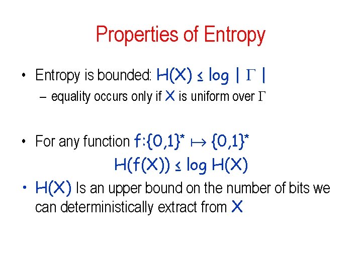
Properties of Entropy • Entropy is bounded: H(X) ≤ log | | – equality occurs only if X is uniform over • For any function f: {0, 1}* H(f(X)) ≤ log H(X) • H(X) Is an upper bound on the number of bits we can deterministically extract from X

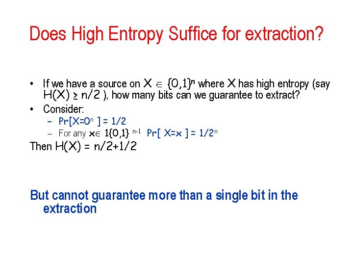
Does High Entropy Suffice for extraction? • If we have a source on X {0, 1}n where X has high entropy (say H(X) ≥ n/2 ), how many bits can we guarantee to extract? • Consider: – Pr[X=0 n ] = 1/2 – For any x 1{0, 1} n-1 Pr[ X=x ] = 1/2 n Then H(X) = n/2+1/2 But cannot guarantee more than a single bit in the extraction

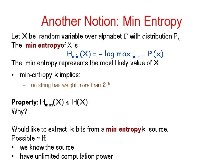
Another Notion: Min Entropy Let X be random variable over alphabet with distribution Px The min entropyof X is Hmin(X) = - log max x P (x) The min entropy represents the most likely value of X • min-entropy k implies: – no string has weight more than 2 -k Property: Hmin(X) ≤ H(X) Why? Would like to extract k bits from a min entropyk source. Possible ~ If: • we know the source • have unlimited computation power

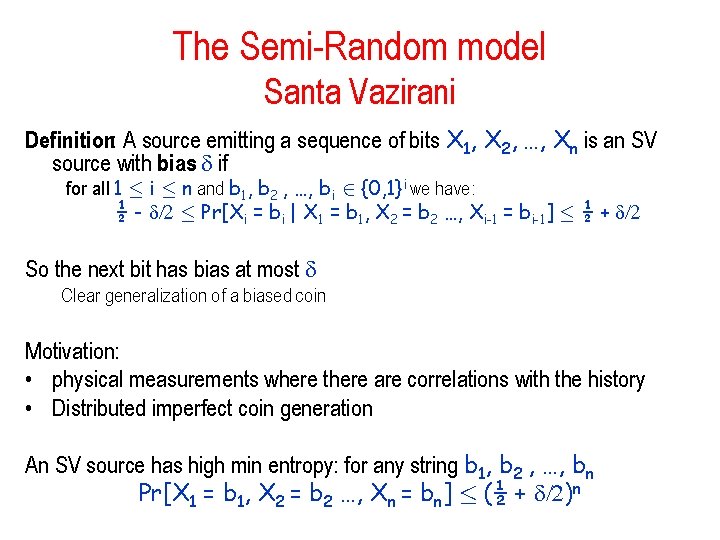
The Semi-Random model Santa Vazirani Definition: A source emitting a sequence of bits X 1, X 2, …, Xn is an SV source with bias if for all 1 · i · n and b 1, b 2 , …, bi 2 {0, 1}i we have: ½ - /2 · Pr[Xi = bi | X 1 = b 1, X 2 = b 2 …, Xi-1 = bi-1] · ½ + /2 So the next bit has bias at most Clear generalization of a biased coin Motivation: • physical measurements where there are correlations with the history • Distributed imperfect coin generation An SV source has high min entropy: for any string b 1, b 2 , …, bn Pr[X 1 = b 1, X 2 = b 2 …, Xn = bn] · (½ + /2)n

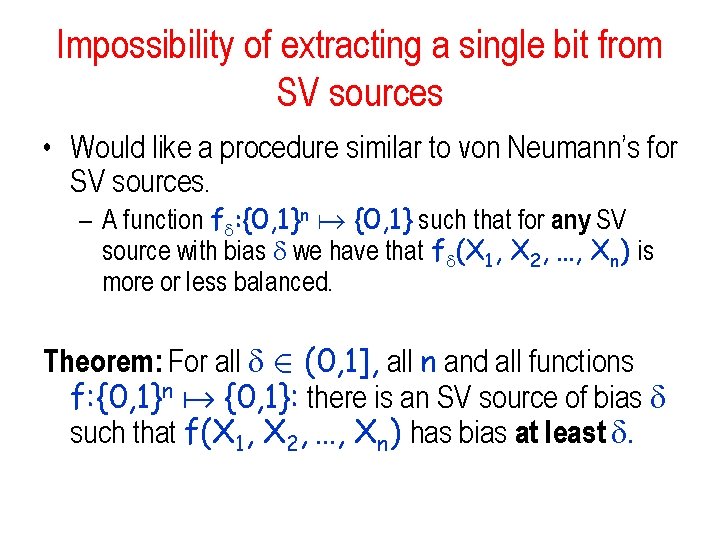
Impossibility of extracting a single bit from SV sources • Would like a procedure similar to von Neumann’s for SV sources. – A function f : {0, 1}n {0, 1} such that for any SV source with bias we have that f (X 1, X 2, …, Xn) is more or less balanced. Theorem: For all 2 (0, 1], all n and all functions f: {0, 1}n {0, 1}: there is an SV source of bias such that f(X 1, X 2, …, Xn) has bias at least .

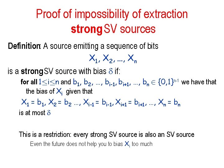
Proof of impossibility of extraction strong SV sources Definition: A source emitting a sequence of bits X 1, X 2, …, Xn is a strong SV source with bias if: for all 1·i·n and b 1, b 2, …, bi-1, bi+1, …, bn 2 {0, 1}n-1 we have that the bias of Xi given that X 1 = b 1, X 2 = b 2 …, Xi-1 = bi-1, Xi+1 = bi+1, …, Xn = bn is at most This is a restriction: every strong SV source is also an SV source Even the future does not help you to bias Xi too much

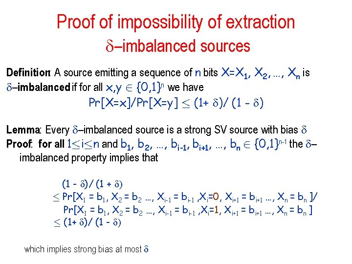
Proof of impossibility of extraction –imbalanced sources Definition: A source emitting a sequence of n bits X=X 1, X 2, …, Xn is –imbalanced if for all x, y 2 {0, 1}n we have Pr[X=x]/Pr[X=y] · (1+ )/ (1 - ) Lemma: Every –imbalanced source is a strong SV source with bias Proof: for all 1·i·n and b 1, b 2, …, bi-1, bi+1, …, bn 2 {0, 1}n-1 the – imbalanced property implies that (1 - )/ (1 + ) · Pr[X 1 = b 1, X 2 = b 2 …, Xi-1 = bi-1 , Xi=0, Xi+1 = bi+1 …, Xn = bn ]/ Pr[X 1 = b 1, X 2 = b 2 …, Xi-1 = bi-1 , Xi=1, Xi+1 = bi+1 …, Xn = bn ] · (1+ )/ (1 - ) which implies strong bias at most

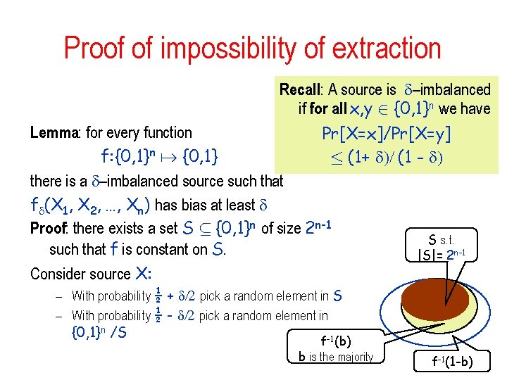
Proof of impossibility of extraction Recall: A source is –imbalanced if for all x, y 2 {0, 1}n we have Lemma: for every function Pr[X=x]/Pr[X=y] f: {0, 1}n {0, 1} · (1+ )/ (1 - ) there is a –imbalanced source such that f (X 1, X 2, …, Xn) has bias at least Proof: there exists a set S µ {0, 1}n of size 2 n-1 S s. t. such that f is constant on S. |S|= 2 n-1 Consider source X: – With probability ½ + /2 pick a random element in S – With probability ½ - /2 pick a random element in {0, 1}n /S -1 f (b) b is the majority f-1(1 -b)

Extractors • So if extraction from SV is impossible should we simply give up? • No: use randomness! Make sure you are using much less randomness than you are getting out

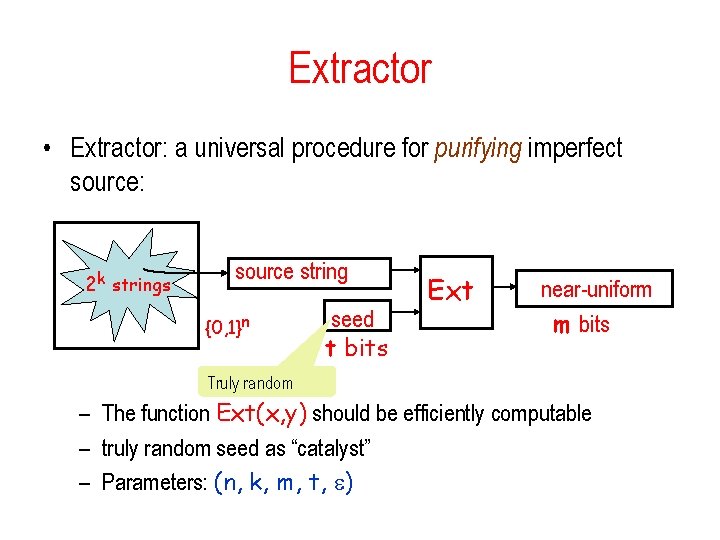
Extractor • Extractor: a universal procedure for purifying imperfect source: 2 k strings source string {0, 1}n seed t bits Ext near-uniform m bits Truly random – The function Ext(x, y) should be efficiently computable – truly random seed as “catalyst” – Parameters: (n, k, m, t, )

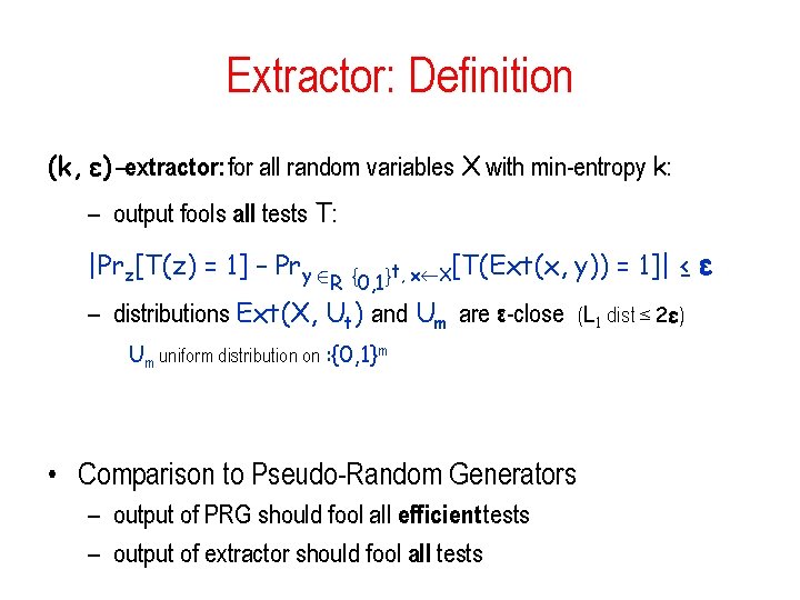
Extractor: Definition (k, ε)-extractor: for all random variables X with min-entropy k: – output fools all tests T: |Prz[T(z) = 1] – Pry 2 t, x X[T(Ext(x, { } R 0, 1 y)) = 1]| ≤ ε – distributions Ext(X, Ut) and Um are ε-close (L 1 dist ≤ 2ε) Um uniform distribution on : {0, 1}m • Comparison to Pseudo-Random Generators – output of PRG should fool all efficient tests – output of extractor should fool all tests

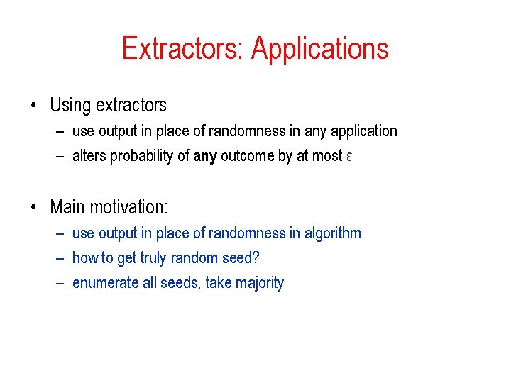
Extractors: Applications • Using extractors – use output in place of randomness in any application – alters probability of any outcome by at most ε • Main motivation: – use output in place of randomness in algorithm – how to get truly random seed? – enumerate all seeds, take majority

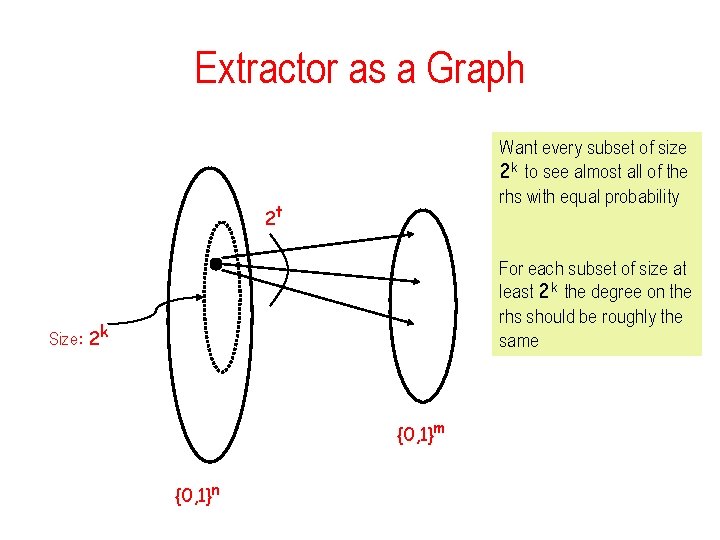
Extractor as a Graph Want every subset of size 2 k to see almost all of the rhs with equal probability 2 t For each subset of size at least 2 k the degree on the rhs should be roughly the same Size: 2 k {0, 1}m {0, 1}n

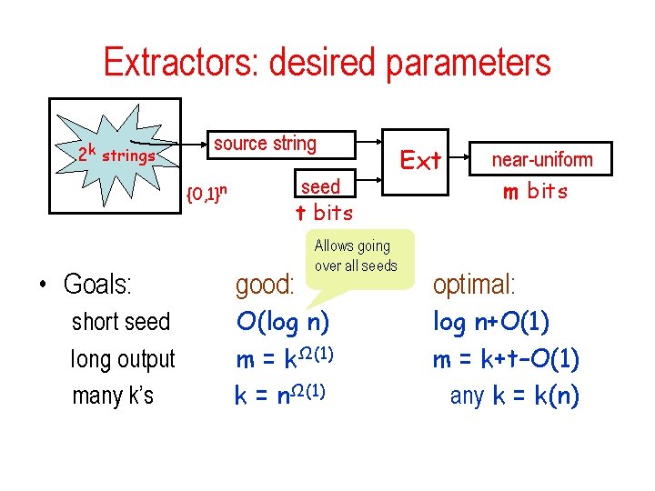
Extractors: desired parameters 2 k strings source string seed t bits {0, 1}n • Goals: short seed long output many k’s good: Allows going over all seeds O(log n) m = kΩ(1) k = nΩ(1) Ext near-uniform m bits optimal: log n+O(1) m = k+t–O(1) any k = k(n)

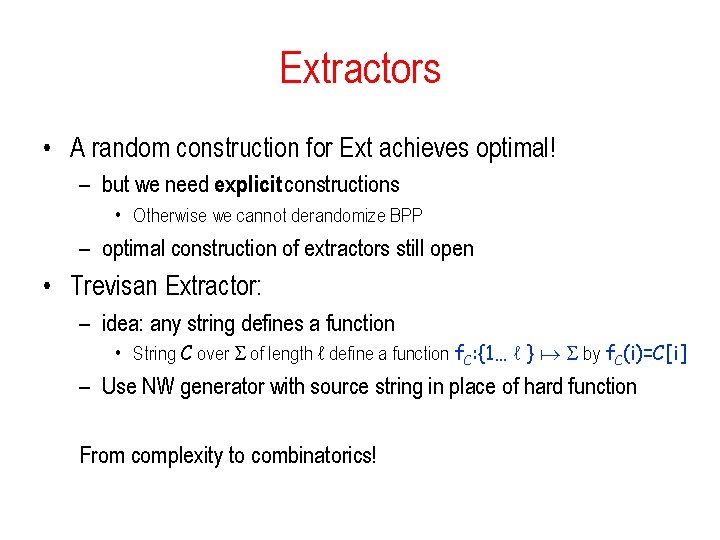
Extractors • A random construction for Ext achieves optimal! – but we need explicit constructions • Otherwise we cannot derandomize BPP – optimal construction of extractors still open • Trevisan Extractor: – idea: any string defines a function • String C over of length ℓ define a function f. C: {1… ℓ } by f. C(i)=C[i] – Use NW generator with source string in place of hard function From complexity to combinatorics!

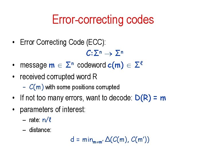
Error-correcting codes • Error Correcting Code (ECC): C: Σn • message m Σn codeword c(m) Σℓ • received corrupted word R – C(m) with some positions corrupted • If not too many errors, want to decode: D(R) = m • parameters of interest: – rate: n/ℓ – distance: d = minm m’ Δ(C(m), C(m’))

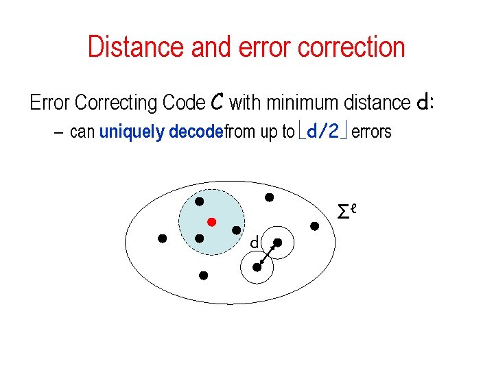
Distance and error correction Error Correcting Code C with minimum distance d: – can uniquely decodefrom up to d/2 errors Σℓ d

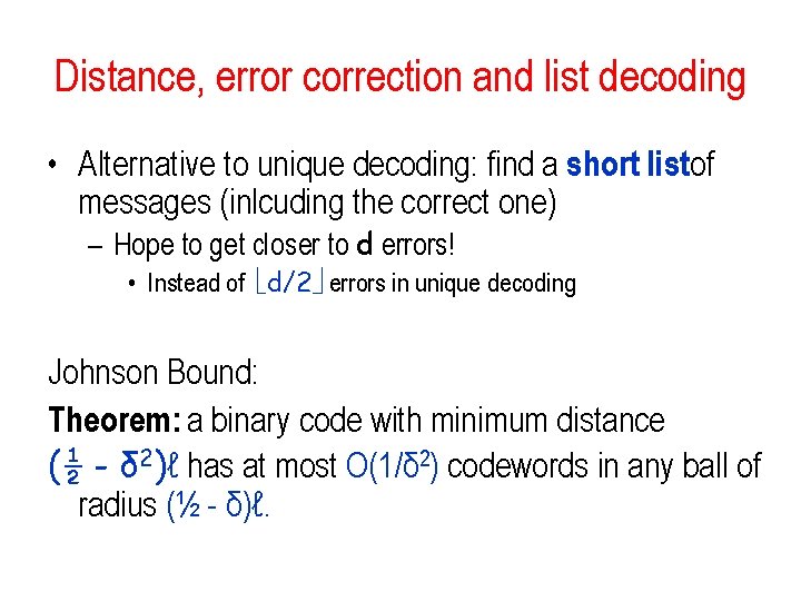
Distance, error correction and list decoding • Alternative to unique decoding: find a short listof messages (inlcuding the correct one) – Hope to get closer to d errors! • Instead of d/2 errors in unique decoding Johnson Bound: Theorem: a binary code with minimum distance (½ - δ 2)ℓ has at most O(1/δ 2) codewords in any ball of radius (½ - δ)ℓ.

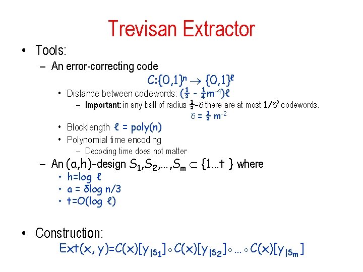
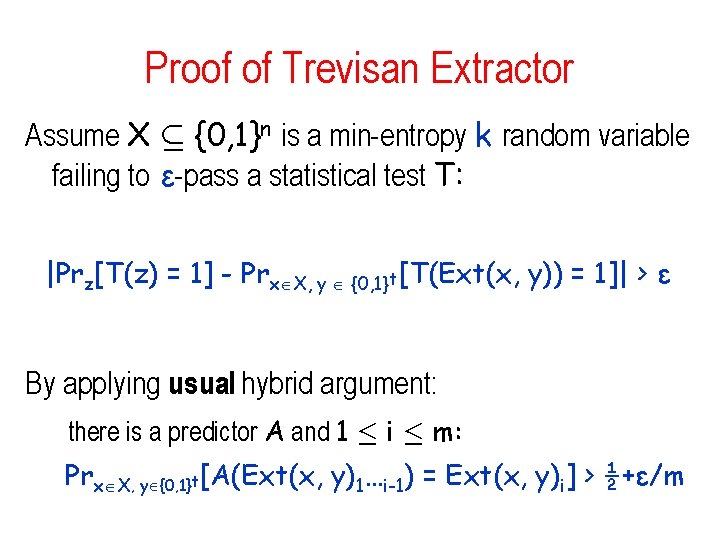
Trevisan Extractor • Tools: – An error-correcting code C: {0, 1}n {0, 1}ℓ • Distance between codewords: (½ - ¼m-4)ℓ – Important: in any ball of radius ½- there at most 1/ 2 codewords. = ½ m-2 • Blocklength ℓ = poly(n) • Polynomial time encoding – Decoding time does not matter – An (a, h)-design S 1, S 2, …, Sm {1…t } where • h=log ℓ • a = δlog n/3 • t=O(log ℓ) • Construction: Ext(x, y)=C(x)[y|S 1]◦C(x)[y|S 2]◦…◦C(x)[y|Sm]

Trevisan Extractor Ext(x, y)=C(x)[y|S 1]◦C(x)[y|S 2]◦…◦C(x)[y|Sm] C(x): 010100101111101010111001010 seed y Theorem: Ext is an extractor for min-entropy k = nδ, with – output length m = k 1/3 – seed length t = O(log ℓ ) = O(log n) – error ε ≤ 1/m

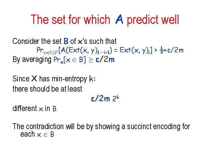
Proof of Trevisan Extractor Assume X µ {0, 1}n is a min-entropy k random variable failing to ε-pass a statistical test T: |Prz[T(z) = 1] - Prx X, y {0, 1}t[T(Ext(x, y)) = 1]| > ε By applying usual hybrid argument: there is a predictor A and 1 · i · m: Prx X, y {0, 1}t[A(Ext(x, y)1…i-1) = Ext(x, y)i] > ½+ε/m

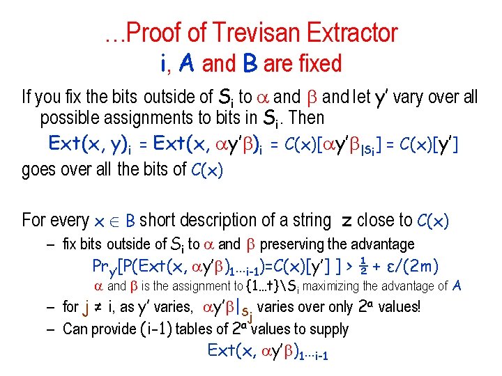
The set for which A predict well Consider the set B of x’s such that Pry {0, 1}t[A(Ext(x, y)1…i-1) = Ext(x, y)i] > ½+ε/2 m By averaging Prx[x 2 B] ¸ ε/2 m Since X has min-entropy k: there should be at least ε/2 m 2 k different x in B The contradiction will be by showing a succinct encoding for each x 2 B

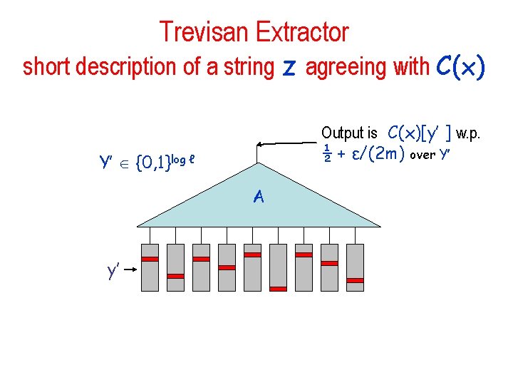
…Proof of Trevisan Extractor i, A and B are fixed If you fix the bits outside of Si to and let y’ vary over all possible assignments to bits in Si. Then Ext(x, y)i = Ext(x, y’ )i = C(x)[ y’ |Si] = C(x)[y’] goes over all the bits of C(x) For every x 2 B short description of a string z close to C(x) – fix bits outside of Si to and preserving the advantage Pry’[P(Ext(x, y’ )1…i-1)=C(x)[y’] ] > ½ + ε/(2 m) and is the assignment to {1…t}Si maximizing the advantage of A – for j ≠ i, as y’ varies, y’ |Sj varies over only 2 a values! – Can provide (i-1) tables of 2 a values to supply Ext(x, y’ )1…i-1

Trevisan Extractor short description of a string z agreeing with C(x) Output is C(x)[y’ ] w. p. ½ + ε/(2 m) over Y’ Y’ {0, 1}log ℓ A y’

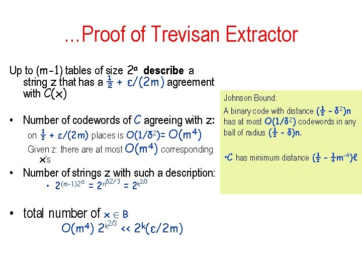
…Proof of Trevisan Extractor Up to (m-1) tables of size 2 a describe a string z that has a ½ + ε/(2 m) agreement with C(x) • Number of codewords of C agreeing with z: on ½ + ε/(2 m) places is O(1/δ 2)= O(m 4) Given z: there at most O(m 4) corresponding x’s • Number of strings z with such a description: a δ 2/3 • 2(m-1)2 = 2 n 2/3 = 2 k • total number of x 2 B O(m 4) 2 k 2/3 << 2 k(ε/2 m) Johnson Bound: A binary code with distance (½ - δ 2)n has at most O(1/δ 2) codewords in any ball of radius (½ - δ)n. • C has minimum distance (½ - ¼m-4)ℓ

Conclusion • Given a source of n random bits with min entropy k which is n (1) it is possible to run any BPP algorithm using the source and obtain the correct answer with high probability Even though extracting even a single bit may be impossible

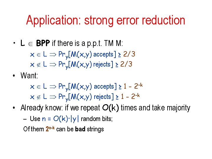
Application: strong error reduction • L BPP if there is a p. p. t. TM M: x L Pry[M(x, y) accepts] ≥ 2/3 x L Pry[M(x, y) rejects] ≥ 2/3 • Want: x L Pry[M(x, y) accepts] ≥ 1 - 2 -k x L Pry[M(x, y) rejects] ≥ 1 - 2 -k • Already know: if we repeat O(k) times and take majority – Use n = O(k)·|y| random bits; Of them 2 n-k can be bad strings

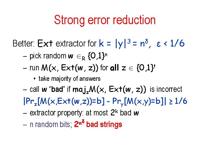
Strong error reduction Better: Ext extractor for k = |y|3 = nδ, ε < 1/6 – pick random w R {0, 1}n – run M(x, Ext(w, z)) for all z {0, 1}t • take majority of answers – call w “bad” if majz. M(x, Ext(w, z)) is incorrect |Prz[M(x, Ext(w, z))=b] - Pry[M(x, y)=b]| ≥ 1/6 – extractor property: at most 2 k bad w δ n – n random bits; 2 bad strings

References • Theory of cryptographic Pseudo-randomness developed by: – Blum and Micali, next bit test, 1982 – Computational indistinguishability, Yao, 1982, • The NW generator: – Nisan and Wigderson, Hardness vs. Randomness, JCSS, 1994. – Some of the slides on the topic: Chris Umans’ course Lecture 9