Complexity Theory Lecture 13 Lecturer Moni Naor Recap

Complexity Theory Lecture 13 Lecturer: Moni Naor

Recap Last week: Finish Hardness and Randomness Circuit Complexity The class NC Formulae = NC 1 Lower bound for. Andreev’s function Communication characterization of depth This Week: P-Completeness of inverting NC 0 Permutations Communication characterization of depth Lower bound on monotonest-connectivity Some functions in NC 0 P Addition Multiplication of n numbers Division

Two Surveys on Extractors • Noam Nisan, Amnon Ta-Shma: . Extracting Randomness: A Survey and New Constructions 1999, (predates Trevisan) • R. Shaltiel, Recent developments in Extractors, 2002, www. wisdom. weizmann. ac. il/~ronens/papers/survey. ps Some of the slides based on C. Umans course

Circuit Complexity • We will consider several issues regarding circuit complexity

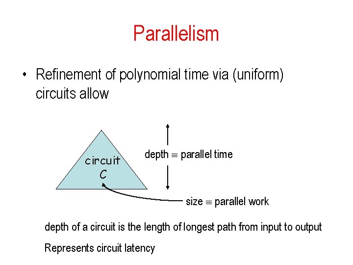
Parallelism • Refinement of polynomial time via (uniform) circuits allow circuit C depth parallel time size parallel work depth of a circuit is the length of longest path from input to output Represents circuit latency

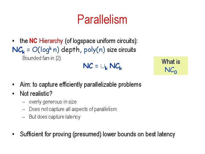
Parallelism • the NC Hierarchy (of logspace uniform circuits): NCk = O(logk n) depth, poly(n) size circuits Bounded fan-in (2) NC = [k NCk What is NC 0 • Aim: to capture efficiently parallelizable problems • Not realistic? – overly generous in size – Does not capture all aspects of parallelism – But does capture latency • Sufficient for proving (presumed) lower bounds on best latency

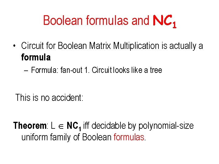
Boolean formulas and NC 1 • Circuit for Boolean Matrix Multiplication is actually a formula. – Formula: fan-out 1. Circuit looks like a tree This is no accident: Theorem: L NC 1 iff decidable by polynomial-size uniform family of Boolean formulas.

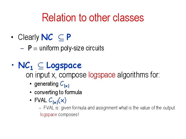
Relation to other classes • Clearly NC µ P – P uniform poly-size circuits • NC 1 µ Logspace on input x, compose logspace algorithms for: • generating C|x| • converting to formula • FVAL C|x|(x) – FVAL is: given formula and assignment what is the value of the output logspace composes!

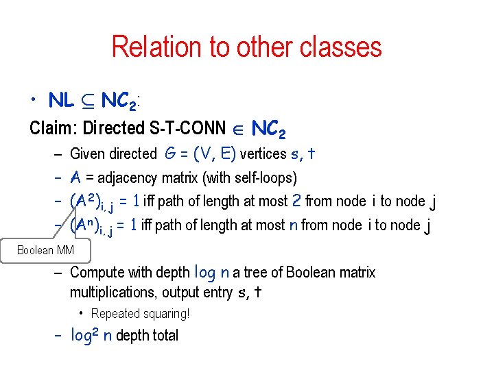
Relation to other classes • NL µ NC 2: Claim: Directed S-T-CONN NC 2 – – Given directed G = (V, E) vertices s, t A = adjacency matrix (with self-loops) (A 2)i, j = 1 iff path of length at most 2 from node i to node j (An)i, j = 1 iff path of length at most n from node i to node j Boolean MM – Compute with depth log n a tree of Boolean matrix multiplications, output entry s, t • Repeated squaring! – log 2 n depth total

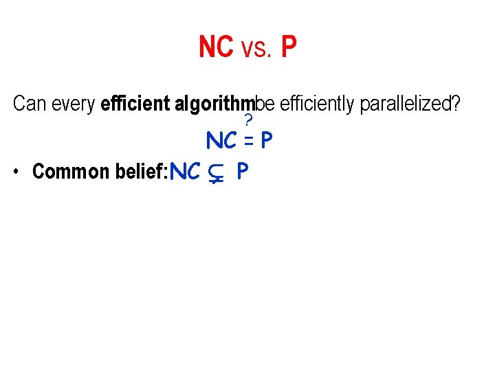
NC vs. P Can every efficient algorithmbe efficiently parallelized? ? NC = P • Common belief: NC ( P

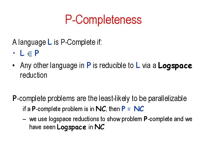
P-Completeness A language L is P-Complete if: • L 2 P • Any other language in P is reducible to L via a Logspace reduction P-complete problems are the least-likely to be parallelizable if a P-complete problem is in NC, then P = NC – we use logspace reductions to show problem P-complete and we have seen Logspace in NC

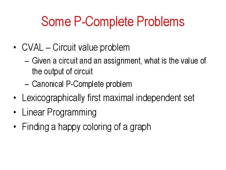
Some P-Complete Problems • CVAL – Circuit value problem – Given a circuit and an assignment, what is the value of the output of circuit – Canonical P-Complete problem • Lexicographically first maximal independent set • Linear Programming • Finding a happy coloring of a graph

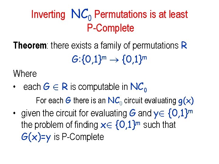
Inverting NC 0 Permutations is at least P-Complete Theorem: there exists a family of permutations R G: {0, 1}m Where • each G 2 R is computable in NC 0 For each G there is an NC 0 circuit evaluating g(x) • given the circuit for evaluating G and y 2 {0, 1}m the problem of finding x 2 {0, 1}m such that G(x)=y is P-Complete

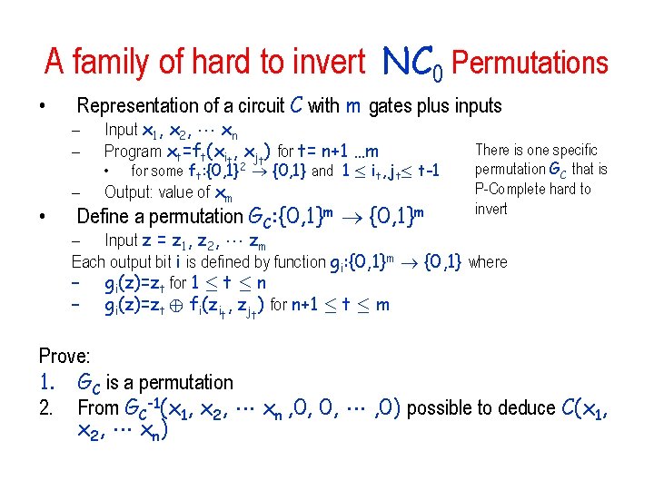
A family of hard to invert NC 0 Permutations • • Representation of a circuit C with m gates plus inputs – – Input x 1, x 2, xn Program xt=ft(xit, xjt) for t= n+1 …m – Output: value of xm • for some ft: {0, 1}2 {0, 1} and 1 · it, jt· t-1 Define a permutation GC: {0, 1}m There is one specific permutation GC that is P-Complete hard to invert – Input z = z 1, z 2, zm Each output bit i is defined by function gi: {0, 1}m {0, 1} where – gi(z)=zt for 1 · t · n – gi(z)=zt © fi(zit, zjt) for n+1 · t · m Prove: 1. GC is a permutation 2. From GC-1(x 1, x 2, xn , 0, 0, , 0) possible to deduce C(x 1, x 2, x n)

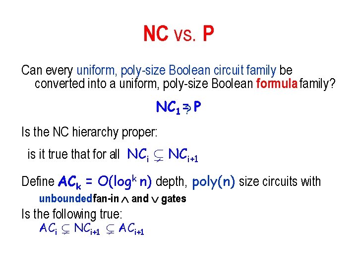
NC vs. P Can every uniform, poly-size Boolean circuit family be converted into a uniform, poly-size Boolean formula family? NC 1 =? P Is the NC hierarchy proper: is it true that for all NCi ( NCi+1 Define ACk = O(logk n) depth, poly(n) size circuits with unbounded fan-in and gates Is the following true: ACi ( NCi+1 ( ACi+1

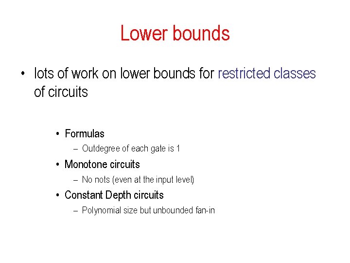
Lower bounds • lots of work on lower bounds for restricted classes of circuits • Formulas – Outdegree of each gate is 1 • Monotone circuits – No nots (even at the input level) • Constant Depth circuits – Polynomial size but unbounded fan-in

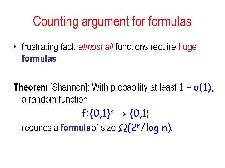
Counting argument formulas • frustrating fact: almost all functions require huge formulas Theorem [Shannon]: With probability at least 1 – o(1), a random function f: {0, 1}n {0, 1} requires a formula of size Ω(2 n/log n).

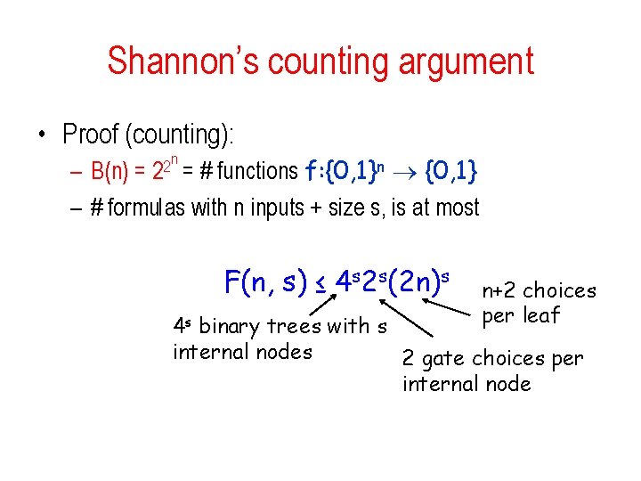
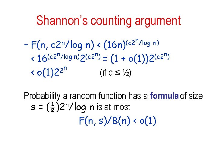
Shannon’s counting argument • Proof (counting): n 2 2 = – B(n) = # functions f: {0, 1}n {0, 1} – # formulas with n inputs + size s, is at most F(n, s) ≤ 4 s 2 s(2 n)s n+2 choices per leaf 4 s binary trees with s internal nodes 2 gate choices per internal node

Shannon’s counting argument n/log n) (c 2 (16 n) – F(n, n) < n/log n) (c 2 n) n) (c 2 < 16 2 = (1 + o(1))2 n 2 < o(1)2 (if c ≤ ½) c 2 n/log Probability a random function has a formula of size s = (½)2 n/log n is at most F(n, s)/B(n) < o(1)

Andreev’s function • best lower bound formulas: Theorem (Andreev, Hastad ‘ 93): the Andreev function requires ( , , )-formulas of size at Ω(n 3 -o(1)).

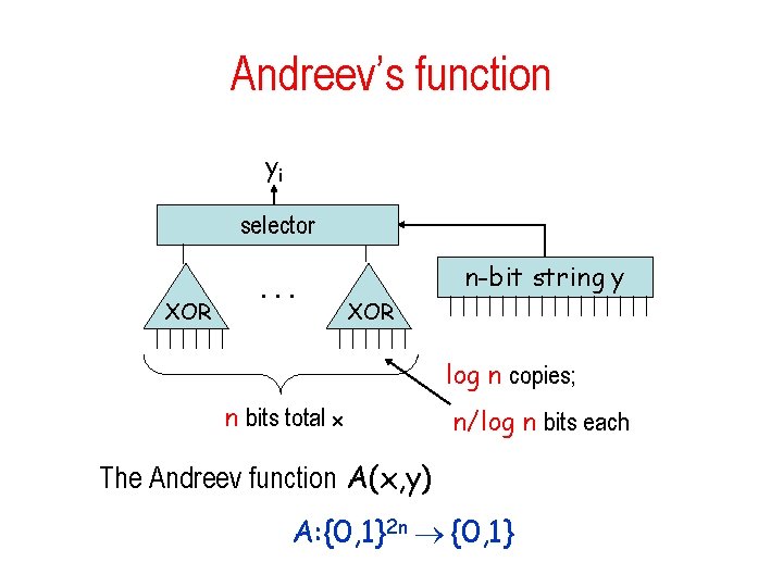
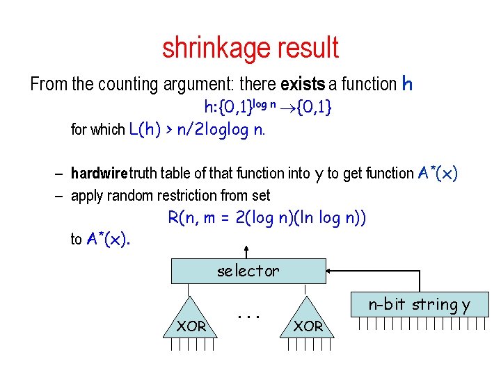
Andreev’s function yi selector XOR . . . n-bit string y XOR log n copies; n bits total x n/log n bits each The Andreev function A(x, y) A: {0, 1}2 n {0, 1}

Andreev’s function Theorem: the Andreev function requires ( , , )-formulas of size at Ω(n 3 -o(1)). First show Ω(n 2 -o(1)). Two important ideas: • Random restrictions • Using the existential counting lower bounds on a smaller domain

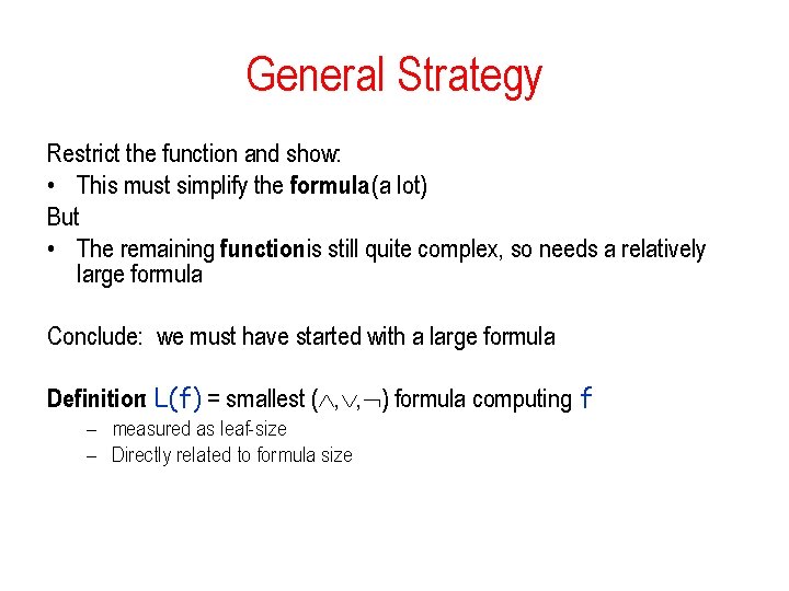
General Strategy Restrict the function and show: • This must simplify the formula (a lot) But • The remaining function is still quite complex, so needs a relatively large formula Conclude: we must have started with a large formula Definition: L(f) = smallest ( , , ) formula computing f – measured as leaf-size – Directly related to formula size

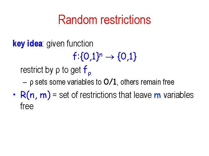
Random restrictions key idea: given function f: {0, 1}n {0, 1} restrict by ρ to get fρ – ρ sets some variables to 0/1, others remain free • R(n, m) = set of restrictions that leave m variables free

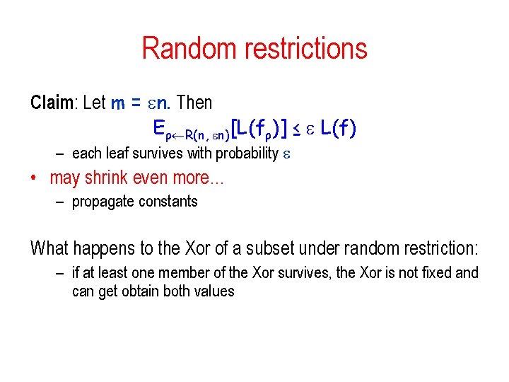
Random restrictions Claim: Let m = n. Then Eρ R(n, n)[L(fρ)] ≤ L(f) – each leaf survives with probability • may shrink even more… – propagate constants What happens to the Xor of a subset under random restriction: – if at least one member of the Xor survives, the Xor is not fixed and can get obtain both values

shrinkage result From the counting argument: there exists a function h h: {0, 1}log n {0, 1} for which L(h) > n/2 loglog n. – hardwire truth table of that function into y to get function A*(x) – apply random restriction from set R(n, m = 2(log n)(ln log n)) to A*(x). selector XOR . . . n-bit string y XOR

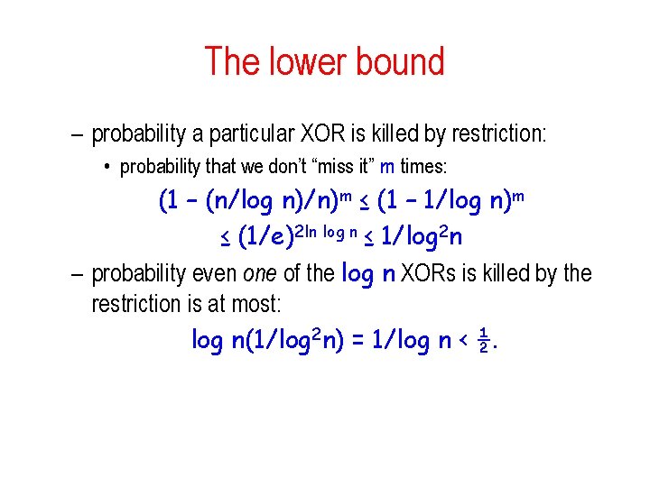
The lower bound – probability a particular XOR is killed by restriction: • probability that we don’t “miss it” m times: (1 – (n/log n)/n)m ≤ (1 – 1/log n)m ≤ (1/e)2 ln log n ≤ 1/log 2 n – probability even one of the log n XORs is killed by the restriction is at most: log n(1/log 2 n) = 1/log n < ½.

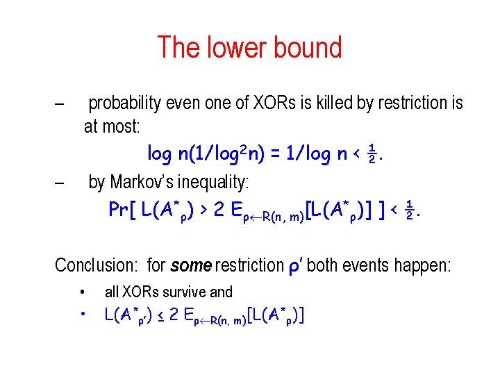
The lower bound – – probability even one of XORs is killed by restriction is at most: log n(1/log 2 n) = 1/log n < ½. by Markov’s inequality: Pr[ L(A*ρ) > 2 Eρ R(n, m)[L(A*ρ)] ] < ½. Conclusion: for some restriction ρ’ both events happen: • • all XORs survive and L(A*ρ’) ≤ 2 Eρ R(n, m)[L(A*ρ)]

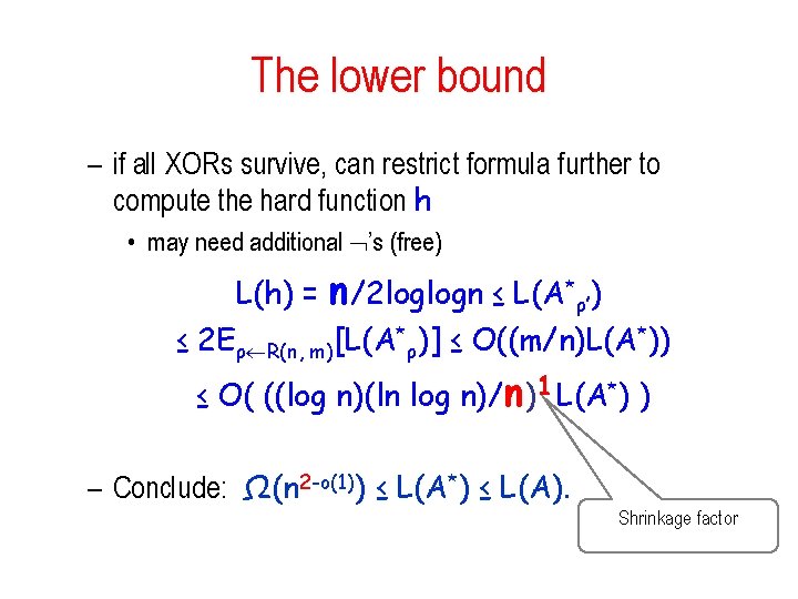
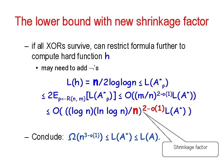
The lower bound – if all XORs survive, can restrict formula further to compute the hard function h • may need additional ’s (free) L(h) = n/2 loglogn ≤ L(A*ρ’) ≤ 2 Eρ R(n, m)[L(A*ρ)] ≤ O((m/n)L(A*)) ≤ O( ((log n)(ln log n)/n)1 L(A*) ) – Conclude: Ω(n 2 -o(1)) ≤ L(A*) ≤ L(A). Shrinkage factor

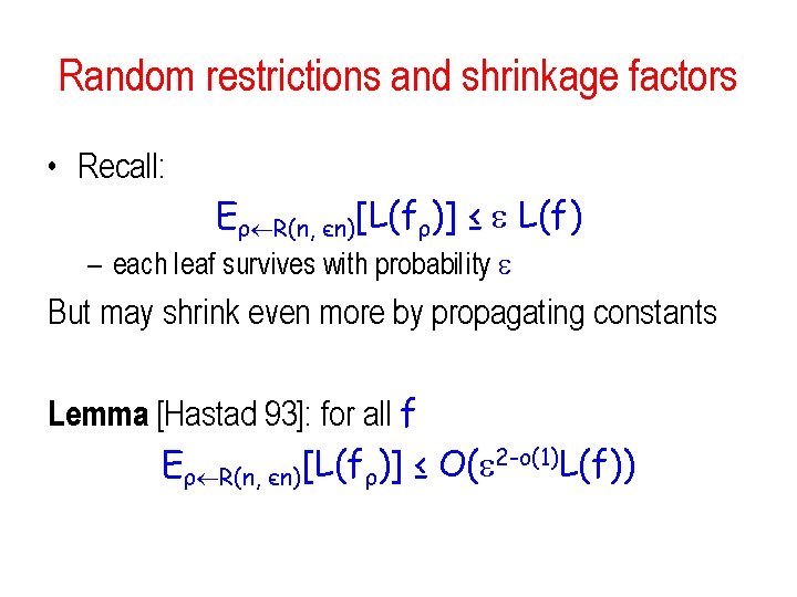
Random restrictions and shrinkage factors • Recall: Eρ R(n, єn)[L(fρ)] ≤ L(f) – each leaf survives with probability But may shrink even more by propagating constants Lemma [Hastad 93]: for all f Eρ R(n, єn)[L(fρ)] ≤ O( 2 -o(1)L(f))

The lower bound with new shrinkage factor – if all XORs survive, can restrict formula further to compute hard function h • may need to add ’s L(h) = n/2 loglogn ≤ L(A*ρ) ≤ 2 Eρ R(n, m)[L(A*ρ)] ≤ O((m/n)2 -o(1)L(A*)) ≤ O( ((log n)(ln log n)/n)2 -o(1) L(A*) ) – Conclude: Ω(n 3 -o(1)) ≤ L(A*) ≤ L(A). Shrinkage factor

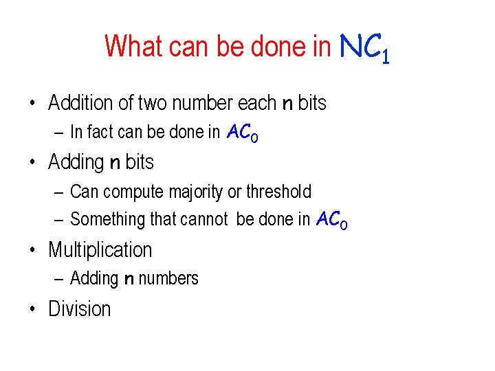
What can be done in NC 1 • Addition of two number each n bits – In fact can be done in AC 0 • Adding n bits – Can compute majority or threshold – Something that cannot be done in AC 0 • Multiplication – Adding n numbers • Division

Two different characterization of NC 1 • Through communication complexity • Through branching programs

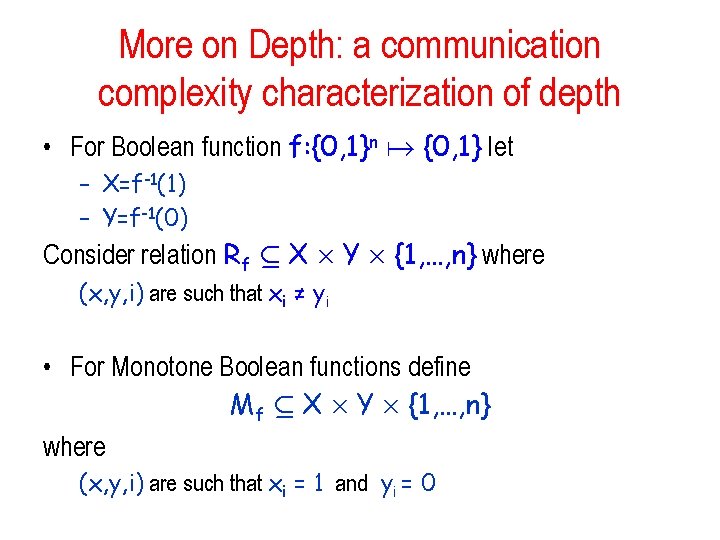
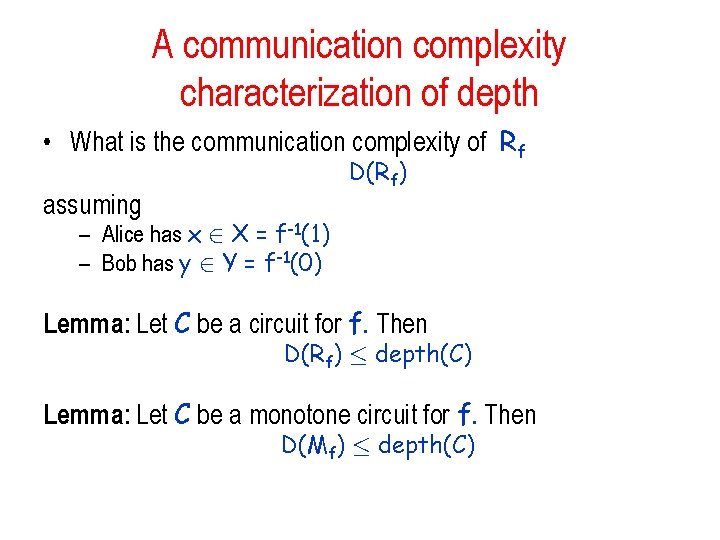
More on Depth: a communication complexity characterization of depth • For Boolean function f: {0, 1}n {0, 1} let – X=f-1(1) – Y=f-1(0) Consider relation Rf µ X £ Y £ {1, …, n} where (x, y, i) are such that xi ≠ yi • For Monotone Boolean functions define Mf µ X £ Y £ {1, …, n} where (x, y, i) are such that xi = 1 and yi = 0

A communication complexity characterization of depth • What is the communication complexity of Rf assuming D(Rf) – Alice has x 2 X = f-1(1) – Bob has y 2 Y = f-1(0) Lemma: Let C be a circuit for f. Then D(Rf) · depth(C) Lemma: Let C be a monotone circuit for f. Then D(Mf) · depth(C)

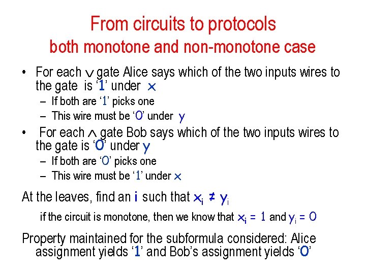
From circuits to protocols both monotone and non-monotone case • For each gate Alice says which of the two inputs wires to the gate is ‘ 1’ under x – If both are ‘ 1’ picks one – This wire must be ‘ 0’ under y • For each gate Bob says which of the two inputs wires to the gate is ‘ 0’ under y – If both are ‘ 0’ picks one – This wire must be ‘ 1’ under x At the leaves, find an i such that xi ≠ yi if the circuit is monotone, then we know that xi = 1 and yi = 0 Property maintained for the subformula considered: Alice assignment yields ‘ 1’ and Bob’s assignment yields ‘ 0’

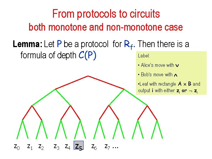
From protocols to circuits both monotone and non-monotone case Lemma: Let P be a protocol for Rf. Then there is a Label: formula of depth C(P) • Alice’s move with • Bob’s move with • Leaf with rectangle A £ B and output i with either zi or zi z 0 z 1 z 2 z 3 z 4 zz 55 z 6 z 7. . .

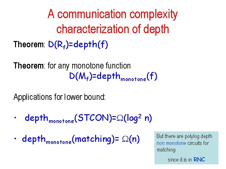
A communication complexity characterization of depth Theorem: D(Rf)=depth(f) Theorem: for any monotone function D(Mf)=depthmonotone(f) Applications for lower bound: • depthmonotone(STCON)= (log 2 n) • depthmonotone(matching)= (n) But there are polylog depth non monotone circuits for matching since it is in RNC

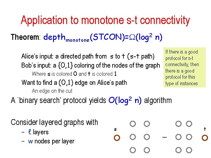
Application to monotone s-t connectivity Theorem: depthmonotone(STCON)= (log 2 n) Alice’s input: a directed path from s to t (s-t path) Bob’s input: a {0, 1} coloring of the nodes of the graph Where s is colored 0 and t is colored 1 Want to find a (0, 1) edge on Alice’s path If there is a good protocol for s-t connectivity, then there is a good protocol for this type of instances An edge on the cut A `binary search’ protocol yields O(log 2 n) algorithm Consider layered graphs with – ℓ layers – w nodes per layer s … t

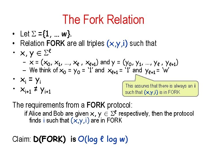
The Fork Relation • Let ={1, … w}. • Relation FORK are all triples (x, y, i) such that • x, y 2 ℓ – x = (x 0, x 1, …, xℓ+1) and y = (y 0, y 1, …, yℓ+1) – We think of x 0 = y 0 = ‘ 1’ and xℓ+1 = ‘ 1’ and yℓ+1 = ‘w’ • xi = y i • xi+1 ≠ yi+1 This assures that there is always an i such that (x, y, i) is in FORK The requirements from a FORK protocol: if Alice and Bob are given x, y 2 ℓ respectively, then the protocol finds i such that (x, y, i) are in FORK Claim: D(FORK) is O(log ℓ log w)

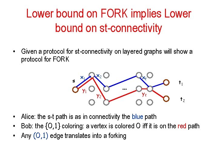
Lower bound on FORK implies Lower bound on st-connectivity • Given a protocol for st-connectivity on layered graphs will show a protocol for FORK s x 1 y 1 x 2 y 2 … xℓ yℓ t 1 t 2 • Alice: the s-t path is as in connectivity the blue path • Bob: the {0, 1} coloring: a vertex is colored 0 iff it is on the red path • Any (0, 1) edge translates into a forking

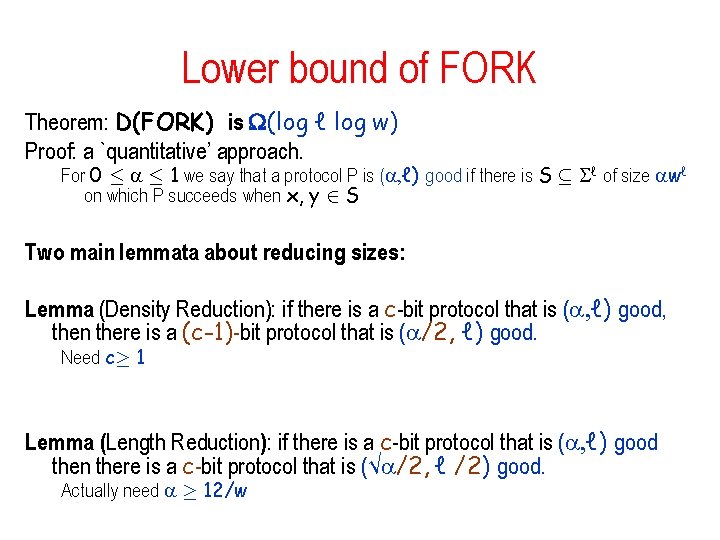
Lower bound of FORK Theorem: D(FORK) is (log ℓ log w) Proof: a `quantitative’ approach. For 0 · · 1 we say that a protocol P is ( , ℓ) good if there is S µ ℓ of size wℓ on which P succeeds when x, y 2 S Two main lemmata about reducing sizes: Lemma (Density Reduction): if there is a c-bit protocol that is ( , ℓ) good, then there is a (c-1)-bit protocol that is ( /2, ℓ) good. Need c¸ 1 Lemma (Length Reduction): if there is a c-bit protocol that is ( , ℓ) good then there is a c-bit protocol that is (√ /2, ℓ /2) good. Actually need ¸ 12/w

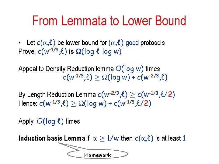
From Lemmata to Lower Bound • Let c( , ℓ) be lower bound for ( , ℓ) good protocols Prove: c(w-1/3, ℓ) is (log ℓ log w) Appeal to Density Reduction lemma O(log w) times c(w-1/3, ℓ) ¸ (log w) + c(w-2/3, ℓ) By Length Reduction Lemma c(w-2/3, ℓ) ¸ c(w-1/3, ℓ/2) Hence: c(w-1/3, ℓ) ¸ (log w) + c(w-1/3, ℓ/2) Apply O(log ℓ) times Induction basis Lemma: if ¸ 1/w then c( , ℓ) is at least 1 Homework

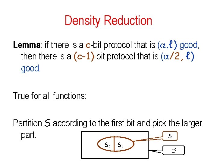
Density Reduction Lemma: if there is a c-bit protocol that is ( , ℓ) good, then there is a (c-1)-bit protocol that is ( /2, ℓ) good. True for all functions: Partition S according to the first bit and pick the larger S part. S 0 S 1 ℓ

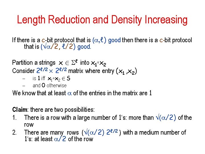
Length Reduction and Density Increasing If there is a c-bit protocol that is ( , ℓ) good then there is a c-bit protocol that is (√ /2, ℓ/2) good. Partition a strings x 2 ℓ into x 1◦x 2 Consider 2ℓ/2 £ 2ℓ/2 matrix where entry (x 1 , x 2) – – is 1 iff x 1◦x 2 2 S and 0 otherwise We know that at least of the entries in the matrix are 1 Claim: there are two possibilities: 1. There is a row with a large number of 1‘s: more than √( /2) of the row 2. There are many rows (√( /2) 2ℓ/2 ) with a medium number of 1‘s: at least /2 of the row

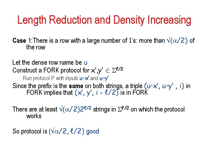
Length Reduction and Density Increasing Case 1: There is a row with a large number of 1‘s: more than √( /2) of the row Let the dense row name be u Construct a FORK protocol for x’, y’ 2 ℓ/2 Run protocol P with inputs u◦x’ and u◦y’ Since the prefix is the same on both strings, a triple (u◦x’, u◦y’ , i) in FORK implies that (x’, y’, i - ℓ/2) is in FORK There at least √( /2)2ℓ/2 strings in ℓ/2 on which the protocol works So protocol is (√ /2, ℓ/2) good

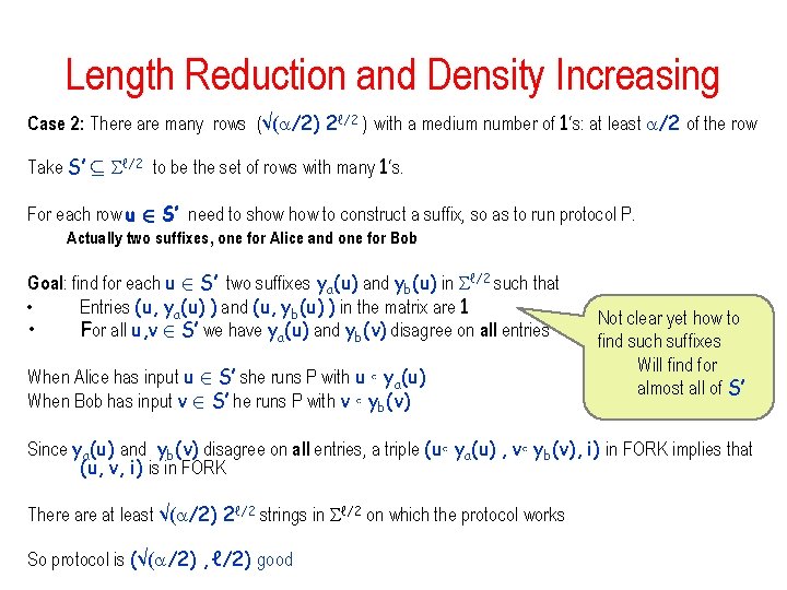
Length Reduction and Density Increasing Case 2: There are many rows (√( /2) 2ℓ/2 ) with a medium number of 1‘s: at least /2 of the row Take S’ µ ℓ/2 to be the set of rows with many 1‘s. For each row u 2 S’ need to show to construct a suffix, so as to run protocol P. Actually two suffixes, one for Alice and one for Bob Goal: find for each u 2 S’ two suffixes ya(u) and yb(u) in ℓ/2 such that • Entries (u, ya(u) ) and (u, yb(u) ) in the matrix are 1 • For all u, v 2 S’ we have ya(u) and yb(v) disagree on all entries When Alice has input u 2 S’ she runs P with u ◦ ya(u) When Bob has input v 2 S’ he runs P with v ◦ yb(v) Not clear yet how to find such suffixes Will find for almost all of S’ Since ya(u) and yb(v) disagree on all entries, a triple (u◦ ya(u) , v◦ yb(v), i) in FORK implies that (u, v, i) is in FORK There at least √( /2) 2ℓ/2 strings in ℓ/2 on which the protocol works So protocol is (√( /2) , ℓ/2) good

Constructing the suffixes • Partition the alphabet for each position 1 · i· ℓ/2 into Ai and Bi – The suffixes ya(u) will be using entries from A 1, A 2 …, Aℓ/2 – The suffixes yb(u) will be using entries from B 1, B 2 …, Bℓ/2 This assures: for all u, v 2 S’: ya(u) and yb(v) disagree on all entries For a random partition for a fixed row u with at least /2 1’s: Think of constructing the partition by: This is a random partition with w/2 entries from each position • pick w/2 random words in ℓ/2 • add for each position random entries so that w/2 entries are chosen altogether Probability not one of the w/2 random words falls into one of the /2 1’s in row u : (1 - /2)w/2 · e- w/4 By symmetry In expectation at most 2 e- w/4 of the rows 2 S’ do not have two proper suffixes

What can be done in NC 1 • Addition of two number each n bits – In fact can be done in AC 0 • Adding n bits – Can compute majority or threshold – Something that cannot be done in AC 0 • Multiplication – Adding n numbers • Multiplying n numbers • Division

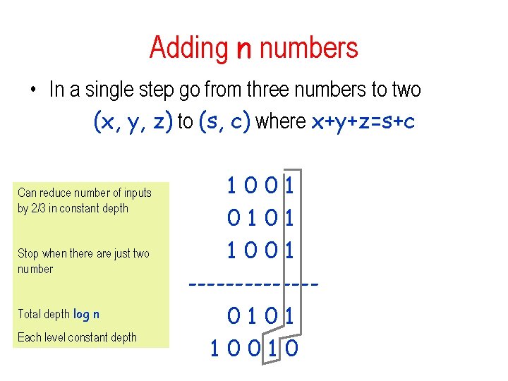
Adding n numbers • In a single step go from three numbers to two (x, y, z) to (s, c) where x+y+z=s+c Can reduce number of inputs by 2/3 in constant depth Stop when there are just two number Total depth log n Each level constant depth 1001 0101 1001 -------0101 10010

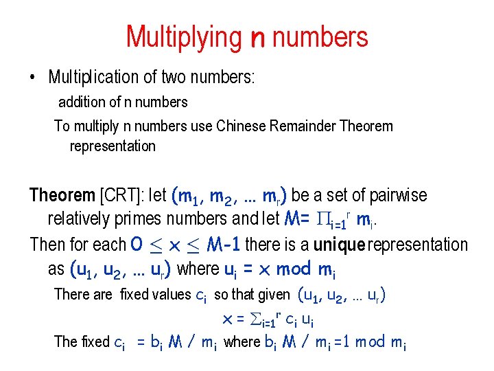
Multiplying n numbers • Multiplication of two numbers: addition of n numbers To multiply n numbers use Chinese Remainder Theorem representation Theorem [CRT]: let (m 1, m 2, … mr) be a set of pairwise relatively primes numbers and let M= i=1 r mi. Then for each 0 · x · M-1 there is a unique representation as (u 1, u 2, … ur) where ui = x mod mi There are fixed values ci so that given (u 1, u 2, … ur) x = i=1 r ci ui The fixed ci = bi M / mi where bi M / mi =1 mod mi

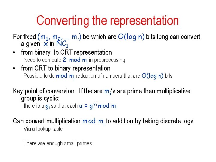
Converting the representation For fixed (m 1, m 2, … mr) be which are O(log n) bits long can convert a given x in NC 1 • from binary to CRT representation Need to compute 2 i mod mj in preprocessing • from CRT to binary representation Possible to do mod mj reduction of numbers that are O(log n) bits Key point of conversion: If the are mi‘s are prime then multiplicative group is cyclic: there is a gi so that each ui = giyi mod mi Can convert multiplication mod mj to addition by taking discrete logs Via a lookup table There are enough small primes

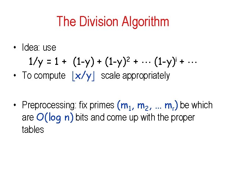
The Division Algorithm • Idea: use 1/y = 1 + (1 -y)2 + (1 -y)i + • To compute bx/yc scale appropriately • Preprocessing: fix primes (m 1, m 2, … mr) be which are O(log n) bits and come up with the proper tables

References • Karchmer and Wigderson, 1988: the communication complexity characterization of depth and s-t connectivity lower bounds Fork is from Grigni and Sipser Raz and Wigderson: depthmonotone(matching)= (n) • Håstad 1987 – Hard to invert Permutations in NC 0. • Beame, Cook and Hoover 1984 – Division in NC 1.