Production and cost analysis Unit 2 Prof Prasanna

Production and cost analysis : Unit 2 Prof Prasanna Shembekar

Production • Process by which resources are transformed in to more useful goods or services • Processing, assembling, producing, manufacturing, extracting, purifying, packaging, storing, transportation, retailing are all productive activities as they add “Value” • Inputs to production are : Land labour capital raw material time and technology. Output is goods or service

Theory of Production • Production is a process that create/adds value or utility • It is the process in which the inputs are converted in to outputs. Inputs • The factors of production such as Land, Labour, Capital, Technology , etc Outputs • The goods and service produced such as Soap, Omni Car , etc

Short run and Long Run • In short run time period supply of some factors is fixed or inelastic. Ex: Land , machinery • In long run all factors are variable except technology • In very long run all factors are variable including technology

Production Function • Production function means the functional relationship between inputs and outputs in the process of production. • It is a technical relation which connects factors inputs used in the production function and the level of outputs Q = f (Land, Labour, Capital, Organization, Technology, etc)

Production function • Overall production function is expressed as: • Q= f (Ld, L, K, M, T, t) Ld= land, L = Labour, K= Capital, M= Machinery, T= Technology, t= time • In general form Q = f (K, L) in long run • Q=f (L) in shot run

Factors of Production Land • Natural resources such as surface, mineral , air, rivers, sea, etc • Free gift of nature, fixed Labour • Mental or physical effort done by a man with the view of Capital • Man made goods used in the production process • Most mobile factor Organization • Entrepreneur or coordinator of all other factors of production

Various concept of production Total Product – Total production done till time using given inputs Average Product- Ratio of Total Product and one variable inputs Marginal Product – The marginal change in output as a result changes in one variable input

Short run Production Function with Labour as Variable factor Labour (L) Capital (K) Total Output (TP) 0 10 0 1 10 10 2 10 30 3 10 4 10 5 10 95 6 10 108 7 10 112 8 10 112 9 10 108 10 10 100 Average Product (AP) 60 Production with One Variable Input 80 Marginal Product (MP)

Short run Production Function with Labour as Variable factor Labour (L) Capital (K) Total Output (TP) Average Product Marginal Product (AP) (MP) 0 10 0 - 1 10 10 2 10 30 15 20 3 10 4 10 80 20 20 5 10 95 19 15 6 10 108 18 13 7 10 112 16 4 8 10 112 14 0 9 10 108 12 -4 10 10 10 -8 60 20 Production with One Variable Input 30

D 112 Output per month Total Product C B 60 A 3 4 8 Labor per month 30 E 20 Average product 10 3 4 8 Labor per month Marginal product

Law of Production Function 1) Laws of Variable proportion- Law of Diminishing Return ( Short run production function with at least one input is variable) 2) Laws of Return to scales – Long run production function with all inputs factors are variable.

1. Law of variable proportion: Short run Production Function • Production function with at least one variable factor keeping the quantities of others inputs as a Fixed. • It shows the input-out put relation when one inputs is variable “When one factor of production is gradually increased keeping other factors constant, marginal product increases up to one stage then it remains constant and if the factor is increased further then the marginal product starts declining ”

Short run Production Function with Labour as Variable factor Labour (L)Land Capital (K) Total Output (TP) Average Product Marginal Product (AP) (MP) 0 10 10 0 - 1 10 10 10 2 10 10 30 15 20 3 10 10 4 10 10 80 20 20 5 10 10 95 19 15 60 20 Production with One Variable Input First Stage 30 6 10 10 108 18 13 7 10 10 112 16 4 8 10 10 112 14 0 9 10 10 108 12 -4 10 100 10 -8 Second Stage Third Stage

D 112 Output per month Total Product C B 60 A 3 4 30 8 Labor per month Second Stage Third Stage E 20 10 Average product First Stage 3 4 8 Labor per month Marginal product

Stages in Law of variable proportion First Stage: Increasing return § § TP increase at increasing rate till the end of the stage. AP also increase and reaches at highest point at the end of the stage. MP also increase at it become equal to AP at the end of the stage. MP>AP Second Stage: Diminishing return § TP increase but at diminishing rate and it reach at highest at the end of the stage. § AP and MP are decreasing but both are positive. § MP become zero when TP is at Maximum, at the end of the stage § MP<AP. Third Stage: Negative return § TP decrease and TP Curve slopes downward § As TP is decreased MP is negative. AP is decreasing but positive.

Where should rational firm produce?

Where should rational firm produce? • Stage I: MP is above AP implies an increase in input increases output in greater proportion. • The firm is not making the best possible use of the fixed factor. • So, the firm has an incentive to increase input until it crosses over to stage II. • Stage III: MP is negative implies contribution of additional labor is negative so the total output decreases. • In this case it will be unwise to employ an additional labor.

• Stage II: MP is below AP implies increase in input increases output in lesser proportion. • A rational producer/firm should produce in stage II.

2. Law of return to scales: Long run Production Function • Explain long run production function when the inputs are changed in the same proportion. • Production function with all factors of productions are variable. . • Show the input-out put relation in the long run with all inputs are variable. “Return to scale refers to the relationship between changes of outputs with proportionate changes in the in all factors of production ”

Law of return to scales: Long run Production Function Labour Capital TP MP 2 1 8 8 4 2 18 10 6 3 30 12 8 4 40 10 10 5 50 10 12 6 60 10 14 7 68 8 16 8 74 6 18 9 78 4 Increasing returns to scale Constant returns to scale Decreasing returns to scale

Law of return to scales: Long run Production Function Inputs 10% increase – Outputs 15% increase Inputs 10% increase – Outputs 10% increase Inputs 10% increase – Outputs 5% increase Increasing returns to scale Constant returns to scale Decreasing returns to scale

Laws of increasing returns to scale • When the combination of factors increases, marginal product increases many folds. • Factors leading to increasing returns ( economies of scale) • Increases degree of specialization • Synergy and higher morale • Effective utilization of resources

Constant returns to scale • When the inputs are doubled, outputs are also doubled. • Production is moving towards point of saturation due to limits of economies of scale. • It may start turning up in to diseconomies of scale. • Region of maximum production

Decreasing returns to scale • This occurs when an increase in all inputs leads to a less than proportional increase in output. • This phenomena happens to increasing diseconomies of scale • More addition to scale leads to inefficient supervision, shortage of raw material, chaos at workplace, social loafing and rivalry among labour

Isoquants • The Greek word ‘iso’ means ‘equal’ or ‘same’ and ‘quant’ is the short form of quantity. Thus an isoquant is a curve along which output is the same. • For the sake of analysis, we are assuming that a producer employs two inputs—labour (L) and capital (K). • A firm can produce a certain amount of a commodity by employing different combinations of labour and capital. • When this information is plotted on a graph paper, we obtain an isoquant.

Iosquants Combination Labour Capital Output level A 20 1 100 unit B 18 2 100 unit C 12 3 100 unit D 9 4 100 unit E 6 5 100 unit F 4 6 100 unit An isoquants represent all those possible combination of two inputs (labour and capital), which is capable to produce an equal level of output.

Iosquants Isoquants or equal product curve Capital 100 unit output Labour An isoquants represent all those possible combination of two inputs (Labour and Capital), which is capable to produce an equal level of output.

Marginal Rate Technical Substitute(MRTS) Isoquants or equal product curve Capital 100 unit output Labour The slop of isoquant is known as Marginal Rate of Technical Substitution (MRTS). It is the rate at which one factors of production is substitute with other factor so that the level of the out put remain the same. MRTS = Changes in Labour / changes in capital

Properties of ISOQUANTS • Negative slope : The slope is negative because the two factors L and K are partially substitutable for each other. • Convex to origin: Due to diminishing marginal rate of substitution D K/ D L goes on reducing at each point • Two isoquants do not intersect each other : Because one cant have two different productions with same combination of factors • Higher production isoquants shift rightwards

Ridge Lines: The Economic Region of Production • Not all points of an isoquant are relevant for production. • One should consider only feasible portions of an isoquant, because no rational producer will produce where marginal product of an input is either zero or negative. • Only the negatively sloped segment of the isoquant is relevant for production or economically feasible. • This is shown in Fig. 3. 5 where

The Lines R & L are the ridge lines outside which production is not feasible. Thus the area that falls within R, L and the isoquant is called economic region of production

LAWS OF RETURNS TO SCALE THROUGH PRODUCTION FUNCTION • Production function is Qx = f ( K, L) • Suppose the scale of inputs is increased by a times and the output increased b times • b. Qx = f(a. K, a. L) = f a (K, L) • If b=a , constant returns to scale • If b> a , increasing returns to scale • If b< a , decreasing returns to scale

Cost concepts • Accounting costs 1. Opportunity and actual costs 2. Business costs and full costs 3. Explicit and implicit or imputed costs 4. Out of pocket and book costs • Analytical costs 1. Fixed and variable costs 2. Total , average and marginal costs 3. Short run and long run costs 4. Incremental and sunk costs 5. Historical and replacement costs 6. Private and social costs

Opportunity cost • Opportunity cost is the expected returns from the second best use of the resources foregone due to the scarcity of resources. • It is also called Alternative cost. It’s an economic cost. • Ex: Suppose that a person has a sum of Rs. 1, 000 from which he can buy either a printing machine or a lathe machine. From printing machine, he expects an annual income of Rs. 20, 000 and from the lathe, Rs. 15, 000. • If he is a profit maximizing investor, he would invest his money in printing machine and forego the expected income from the lathe. • The opportunity cost of his income from printing machine is the expected income from the lathe, i. e. , Rs. 15, 000.

Actual Cost • Actual costs are actually incurred by the firm in payment for labour, material, plant, building, machinery, equipment, travelling and transport, advertisement, etc. • The total money expenses, recorded in the books of accounts are, for all practical purposes, the actual costs. • Actual cost comes under the accounting concept.

Business Costs • Business costs include all the expenses which are incurred to carry out business. • Similar to the actual or real costs. • Business costs “include all the payments and contractual obligations made by the firm together with the book cost of depreciation on plant and equipment”. • These cost concepts are used for calculating business profits and losses and for filling returns for income-tax and also for other legal purposes.

Full costs • Full costs include business costs, opportunity cost and normal profit. • Normal profit is a necessary minimum earning in addition to the opportunity cost, which a firm must get to remain in its present occupation.

EXplicit vs Implicit costs • Explicit costs fall under actual or • Implicit or imputed costs may be business costs entered in the defined as the earning expected from books of accounts. the second best alternative use of resources. • The payments for wages and salaries, materials, license fee, • If an entrepreneur does not utilize his insurance premium, depreciation services in his own business and charges are the examples of works as a manager in some other explicit costs. firm on a salary basis. • These costs involve cash • Implicit costs are not taken into payments and are recorded in account while calculating the loss or normal accounting practices. gains of the business. • But they form an important consideration in whether or not a The explicit and implicit costs factor would remain in its present together make the economic occupation. cost.

• Out of pocket costs involve current cash payments to outsiders • Not all out-of- pocket costs are variable, e. g. , salaries paid to the administrative staff, Neither are they all direct, e. g. , the electric power bill. • Book costs are such as depreciation do not require current cash payments. • Book costs are in some cases variable and in some cases readily traceable, and hence become a part of direct costs. Book costs can be converted into out-of-pocket costs by selling the assets and having them on hire. Rent would then replace depreciation and interest. While undertaking expansion, book costs do not come into the picture until the assets are purchased.

• Fixed costs are those costs which • Variable costs are those are fixed in volume for a certain which vary with the given output. variation in the total output. • Fixed cost does not vary with variation in the output. • They are a function of output. • The costs that do not vary for a certain level of output are known • Variable costs include as fixed cost of raw materials, running cost on fixed • The fixed costs include: capital, such as fuel, – (i) Cost of managerial and repairs, routine administrative staff. maintenance – (ii) Depreciation of machinery, expenditure, direct building and other Axed assets, labour charges and associated with the level of output, and the costs – (iii) Maintenance of land, etc. of all other inputs that • The concept of fixed cost is vary with output. associated with short-run.

Total Cost • Total cost represents the value of the total resource requirement for the production of goods and services. • It refers to the total expenditure, both explicit and implicit, on the resources used to produce a given level of output. • It includes both fixed and variable costs. The total cost for a given output is given by the cost function. TC = FC + VC

• Average cost: • Average cost (AC) is of statistical nature, it is not actual cost. It is obtained by dividing the total cost (TC) by the total output (Q), i. e. • AC = TC / Q = average cost • Marginal cost: • Marginal cost is the addition to the total cost on account of producing an additional unit of the product. • Given the cost function, it may be defined as • MC = TCn – TCn-1 • Total, average and marginal cost concepts are used in economic analysis of firm’s production activities.

Short run and long run costs • Short-run costs vary with the variation in output, the size of the firm remaining the same. • In other words, short-run costs are the same as variable costs. • Long-run costs, on the other hand, are the costs which are incurred on the fixed assets like plant, building, machinery, etc. • Such costs have long-run implication in the sense that these are not used up in the single batch of production. • Long-run costs are, by implication, the same as fixed costs. • In the long-run, however, even the fixed costs become variable costs as the size of the firm or scale of production increases. • Short-run costs are those associated with variables in the utilization of fixed plant or other facilities whereas long-run costs are associated with the changes in the size and kind of plant.

Incremental vs sunk costs • Incremental costs are closely related to the concept of marginal cost but with a relatively wider connotation. • While marginal cost refers to the cost of the marginal unit of output, incremental cost refers to the total additional cost associated with the marginal batch of output. • Incremental costs arise due to the change in product lines, addition or introduction of a new product, replacement of worn out plant and machinery, replacement of old technique of production with a new one, etc. • The Sunk costs are those which cannot be altered, increased or decreased, by varying the rate of output. • For example, once it is decided to make incremental investment expenditure and the funds are allocated and spent, all the preceding costs are considered to be the sunk costs since they accord to the prior commitment • They cannot be revised or reversed or recovered when there is change in market conditions or change in business decisions.

Historical vs replacement costs • Historical costs are those costs of an asset acquired in the past whereas replacement cost refers to the outlay which has to be made for replacing an old asset. These concepts own their significance to unstable nature of price behaviour. • Stable prices over time, other things given, keep historical and replacement costs on par with each other. Instability in asset prices makes the two costs differ from each other. • Historical cost of assets is used for accounting purposes, in the assessment of net worth of the firm. The replacement cost figures in the business decision regarding the renovation of the firm.

• Private costs are those which are actually incurred or provided for by an individual or a firm on the purchase of goods and services from the market. • For a firm, all the actual costs both explicit and implicit are private costs. • Private costs are internalized costs that are incorporated in the firm’s total cost of production. • Social costs on the other hand, refer to the total cost to the society on account of production of a commodity. • Social costs include both private cost and the external cost. • a) The cost of resources for which the firm is not compelled to pay a price, i. e. , atmosphere, rivers, and also for the use of public utility services like roadways, drainage system, etc. • (b) The cost in the form of ‘disutility’ created through air, water and noise pollutions, etc. The costs of category. • (b) Total private and public expenditures incurred to safeguard the individual and public interest against the various kinds of health hazards created by the production system.

The cost function • The relation between cost and its determinants is technically described as the cost function. • C= f (S, Q, P, T …. ) • Where; • C= Cost (Unit or total cost) • S= Size of plant/scale of production • O= Quantity of production • P= Prices of inputs • T= Technology

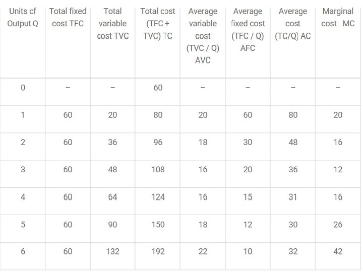
Short Run Table Q TFC TVC TC (TFC+TVC) 0 50 1 50 20 70 2 50 35 85 3 50 60 110 4 50 100 150 5 50 145 195 6 50 190 240 7 50 237 287 8 50 284 334

Short – Run Cost Functions TC TVC Cost TFC B O Q 1 Output The shape : TFC : horizontal straight line TVC: Rises upwards, increases at a decreasing rate upto. Q 1, beyond which it increases at a increasing rate. TC: Same as TVC, the distance between them is constant because of TFC

Cost output relation in Short Run • Total Cost is the summation of Fixed Costs and Variable Costs. • TC=TFC+TVC • Average cost is the total cost per unit. It can be found out as follows. • AC=TC/Q • The total of Average Fixed Cost (TFC/Q) keep coming down as the production is increased. • Marginal Cost is the addition to the total cost due to the production of an additional unit of product. It can be arrived at by dividing the change in total cost by the change in output. • In the short-run there will not be any change in Total Fixed Cost. Hence change in total cost implies change in Total Variable Cost only.

Shape of SRTC curve MC ATC AVC Cost AFC Output

Shape of Short Run Total Cost curve • • The shape of AC curve depend upon AVC and AFC In the beginning both AFC and AVC falls, so AC falls AVC rising and AFC falling, AC still falls But as output increases, a sharp rise AVC offset the fall of AFC and AC start to rise

Short – Run Cost Functions Marginal Cost MC MC < AC = AC falls ( MC pulls the AC down) MC > AC = AC rises ( MC pulls the AC up) MC AC

Long – Run Cost Functions • A firm can vary all its input • The entrepreneur has before him number of alternative plant sizes and levels of output. • In short run the size of the plant ( capital equipment, machinery, land…) are fixed. • In long run the firm can move from one plant to another plant • The LRAC is the least possible average cost production of producing any given level of output when all the inputs are variable.

Derivation of Long Run Average Cost Curve SAC 1 H G Average cost J SAC 2 R L K A B C Output D SAC 3

• In long run firm can vary all its input. • The firm moves from one plant to larger plant if it has to increase its output. • The long run average cost of production is the least possible average cost of producing any given level of output when all the inputs are variable. • The short run average cost curves are called as Plant curves. • Suppose there are only three technically possible size of plant. • The firm can choose among the three possible sizes of plant • Up to OB amount of output, the firm will operate on the SAC 1, though it could produce on SAC 2. • For OA output. It will cost AL per unit cost on SAC 1 curve but it will cost AH if on SAC 2. (AL < AH). • If the firm plans to produce larger output than OB then it has to move to a bigger plant size. • Thus OC if produced on SAC 2 cost CK per unit which is lower than CJ when produced on SAC 1. • If the firm produce output between OB and OD it will employ the plant corresponding to SAC 2.

Long-Run Cost Curve LAC F AC G K M N V Q Output

Long – Run Cost Functions • The LAC is the locus of all the tangency points with the short run average cost curve. • The long run curve is also called as Envelope curve. • LRAC is also called the planning curve: as the firm plans to produce any output in the long run by choosing a plant on the LRAC corresponding to the given output. • Point G lies on the falling portion of SAC 2, the firm is using the given plant below its full capacity. Point F is the minimum point

Why LAC is of U- Shape • Why does LAC fall in the beginning: Economies of Scale - Use of technically efficient Machines - Division of Labour - Indivisibility of factors - Productive capacity of capital equipments rises faster then purchase price - Discounts from bulk purchases - Lower cost of raising funds - Inventory management • Why does LAC rise eventually: Diseconomies of scale - Rise in transportation cost - Input market imperfection - Management co-ordination and control problems - Depletion of raw material

The Concept of Optimum Firm • The best or the ideal size of the firm • The optimum firm is the one which operates on the scale at which, in the existing condition of techniques and organising ability has the lowest average cost of production. • The optimum size of the firm varies a great deal in different industries. – In some industries the minimum point of the long run average cost curve reaches at a comparatively small output ( agriculture, wholesale, retail…) – Optimum size in steel, automobile, heavy industries is very large and the minimum point is reached at a very large output.

The Concept of Optimum Firm LAC AC Output LAC is used as decision making tool to decide which plant should be used. Plant operating at lowest AC is considered

Economies of Scale • The factors which cause the operation of the laws of returns to scale are grouped under economies and diseconomies of scale. • Increasing returns to scale operates because of economies of scale and decreasing returns to scale operates because of diseconomies of scale where economies and diseconomies arise simultaneously.

Continue… • When a firm increases all the factor of production it enjoys the same advantages of economies of production. • The economies of scale are classified as: 1. Internal economies 2. External economies

Internal Economies of Scale • Internal economies are those which arise from the explanation of the plant-size of the firm. • Internal economies of scale may be classified as: 1. Economies in production 2. Economies in marketing 3. Economies in management 4. Economies in transport and storage

Economies in Production • It arises from 1. Technological advantages 2. Advantages of division of labor and specialization

Economies in Marketing • It facilitates through: 1. Large scale purchase of inputs 2. Advertisement economies 3. Economies in large scale distribution 4. Other large-scale economies

Managerial Economies • It achieves through: 1. Specialization in management 2. Mechanization of managerial fucntion

Economies in Transport and Storage • Economies in transportation and storage costs arise from fuller utilization of transport and storage facilities.

External Economies of Scale • External economies to large size firms arise from the discounts available to it due to 1. Large scale purchase of raw materials 2. Large scale acquisition of external finance at low interest 3. Lower advertising rate from advertising media 4. Concessional transport charge on bulk transport 5. Lower wage rates if large scale firm is monopolistic employer of certain kind of specialized labor.

Continue… • External economies of scale are strictly based on experience of large-scale firms or well managed small scale firms. • Economies of scale will not continue for ever. • Expansion in the size of the firms beyond a particular limit, too much specialization, inefficient supervision, improper labor relations etc will lead to diseconomies of scale.