Percolation on Fractal Graphs Surath Fernando Haley Grant

Percolation on Fractal Graphs Surath Fernando, Haley Grant, and Ronilo Ragodos

What is Percolation? Bond Percolation: Start with a fully connected graph of vertices V and edges E, and for each edge e ∈ E, keep e with probability p (and remove e with probability 1 -p). Results in clusters: connected components within the graph Percolation Cluster: Infinite Graph: unique infinite cluster Finite Graph: maximum cluster; spans the boundary of the graph

Critical Probability: pc such that when p < pc the probability of having an infinite cluster is 0, and when p > pc the probability of having an infinite cluster is 1.

Different Fractal Graphs Z x Z lattice (torus structure) SG x SG (double cover) Cell graph x cell graph Also: Magic Carpet Vicsek Fractal SG 3

Z x Z Lattice (torus) Torus identifications - each vertex has 4 neighbors in the original graph (in cross)

SG x SG (double cover) Double cover - each vertex has 8 neighbors (in cross)

Cell Graph (double cover) Each vertex has 6 neighbors (in cross)

Vicsek Set Carpet Magic

SG 3

Locating the Critical Probability Max Cluster Size Max: Second Ratio Count of Spanning Clusters Calibration (Lattice/Torus)

Max Cluster Size: SG Vertex and Lattice SG (Level 3): Probability vs. Max Cluster Size Lattice (100 x 100): Probability vs. Max Cluster Size

Max Cluster Size: Vicsek and Carpet

Max Cluster Size: SG 3 and SG Cell Graph

Max Cluster Size (zoomed in) Zooming in near the critical probability yields an ambiguous region:

Max: Second Ratios: Lattice

Max: Second Ratios: SG

Spanning Clusters On a finite graph with a boundary, define a spanning cluster to be a connected component that intersects two distant sides of the boundary. Boundary of SG x SG Sides: qi x SG and SG x qi , for i = 0, 1, 2. The sides qi x SG and qj x SG are distant sides of the boundary, for i distinct from j. Similarly, SG x qi and SG x qj are distant sides. Boundaries on other product fractals are defined similarly

Spanning Clusters: Lattice

Spanning Clusters: SG

Spanning Clusters: SG Cell

Estimates for Critical Probabilities Figures are based on the ambiguous regions of the spanning clusters graphs. SG x SG: . 187 to. 193 SG Cell x SG Cell: . 265 to. 280 Vicsek x Vicsek: . 350 to. 365 Magic Carpet x Magic Carpet: . 16 to. 19 SG 3 x SG 3: . 16 to. 18 (Lattice: 0. 495 to 0. 505)

Neighbor Distributions As we vary probability, the distribution of number of neighbors over the vertices in the maximal cluster changes. As the probability increases, the graph becomes more highly connected (vertices have more neighbors).

Expected Neighbor Distribution For percolation probability p and graph with N neighbors per vertex (before percolation), the expected value (%) of having k neighbors is: We looked at how our experimental data compared with these expected values, noting that they would never be exactly equal because while ap(0) = (1 - p)N is not zero for 0 < p < 1, in any maximal cluster there are no vertices with zero neighbors.

Neighbor Distribution (Z x Z)

Neighbor Distribution (Z x Z)

Neighbor Distribution (SG x SG)

Neighbor Distribution (SG x SG)

Neighbor Distribution (Cell x Cell)

Neighbor Distribution (Cell x Cell)

Random Walks Random walks on percolation clusters are of interest because cluster graphs are not regular (different vertices have different number of neighbors) Random walk: start at a random vertex in the maximal cluster and move to one of its neighboring vertices with equal probability. Can either be recurrent or transient. ● Recurrent: ○ Infinite - walk returns to starting position infinitely many times with probability 1 ○ Finite - walk returns to starting position at some step **We random walks on maximum clusters to simulate walks on infinite

Random Walks (Z x Z) We know that the Z x Z lattice graph is recurrent at all probabilities (just barely recurrent at p = 1. 0)

Random Walks (SG x SG)

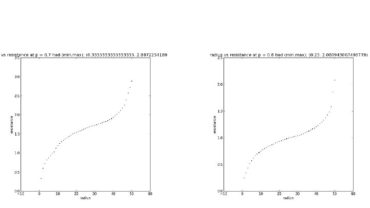
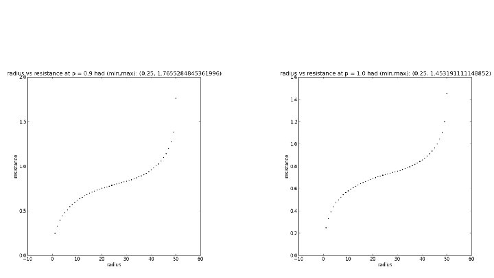
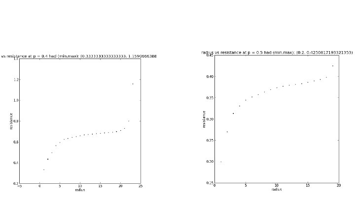
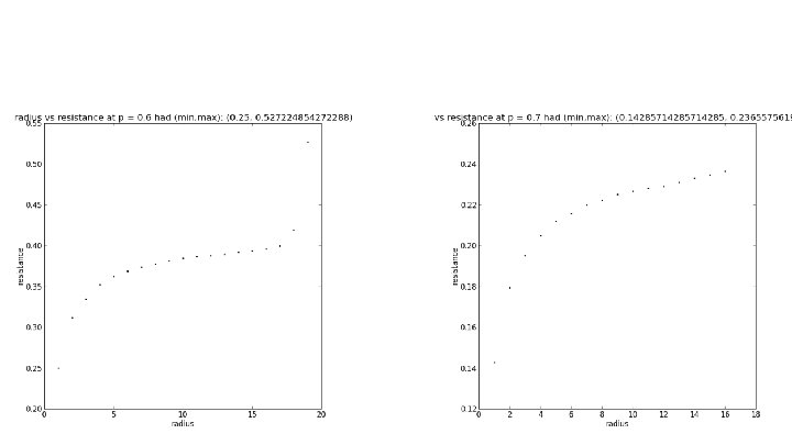
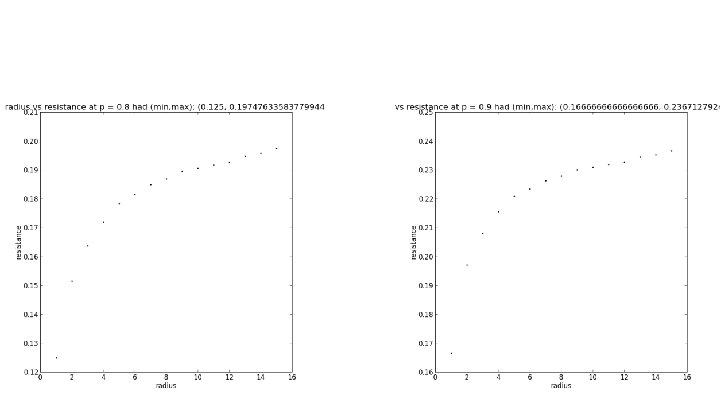
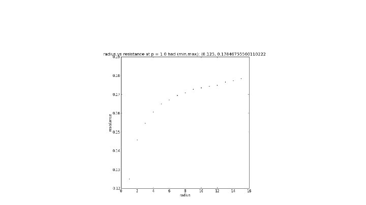
Max Clusters as Electrical Networks We can also model our graphs as electrical networks in order to determine if they are (by nature) recurrent or transient graphs. To do this on our finite graph approximations, we fix a vertex x and call it the origin set up a boundary consisting of vertices a distance r away from x. We give x a voltage of 1 and everything at and beyond the boundary a voltage of 0. The other voltages can be obtained via a system of equations. As we increase r, we take note of the resulting effective resistance Plotting r vs Reff, we would say the graph is recurrent if Reff goes to infinity and transient if it stays bounded. In this model, graph edges with source/target pairs (x, y) are resistors with resistance R(x, y) = 1 / Ε(u) where Ε(u) is the graph energy Ε(u) = ∑a~b(u(a) - u(b))2.

r vs. Effective Resistance on the 2 D Torus Graph

r vs. Effective Resistance on the full 3 D Torus Graph

r vs. Effective Resistance on SG X SG

Is it safe to say there exists a phase transition? Probably, but there are many complications. Many of parameters to vary makes these experiments very computationally expensive Graph approximation level Value of p Number of clusters to create at a given level and probability p Parameters within each experiment (e. g. number of walks to do)

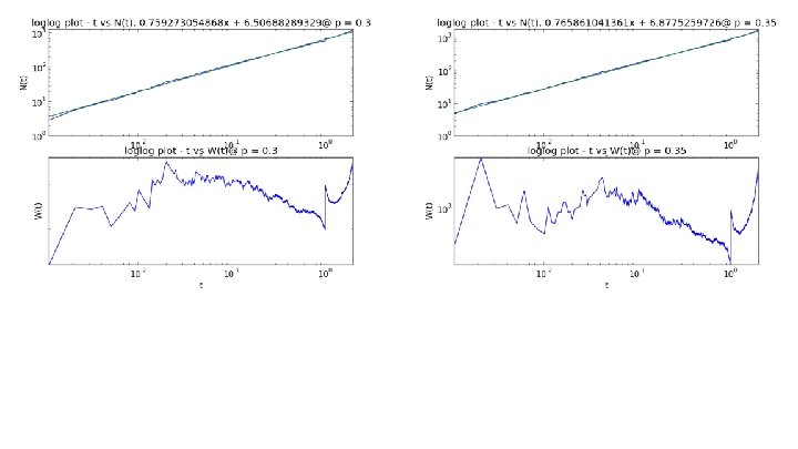
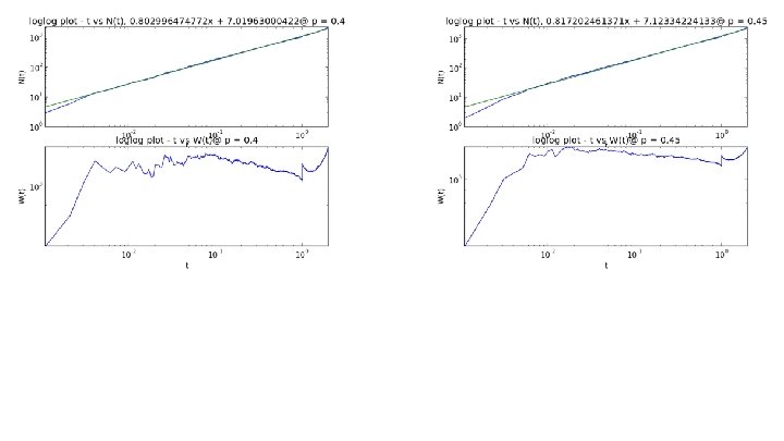
Eigenvalue Counting Function and Weyl Ratio We begin with the regular graph Laplacian matrix G, which is like the adjacency matrix, but with node degrees on the diagonal and edges represented by -1. In other words, it is G = D - A, where D is the degree matrix and A is the adjacency matrix. We then obtain the probabilistic graph laplacian as P = D-1 G. Now define the Eigenvalue counting function N(t) = #{λj ≤t}. If we plot t vs. N(t) log-log and see a linear trend, we can take this as evidence of power law behaviour. Using a linear fit of the log-log plot, we then take the slope to be the associated power law exponent α. We then can compute the Weyl Ratio W(t) = N(t) / tα.

Characterization of the eigenvalues It’s difficult to see (especially on higher levels of SG), but there are gaps in the spectrum 0 ≤ �� ≤ 2 �� = 1 has notably high multiplicity at some levels of p �� = 1. 5 also has notable multiplicity, but to a lesser degree

Plots for SG X SG

On the Torus Graph

On the Cell Graph version of SG X SG

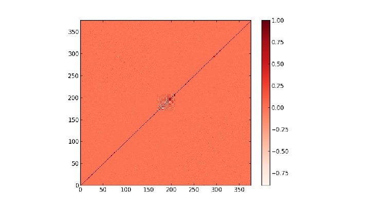
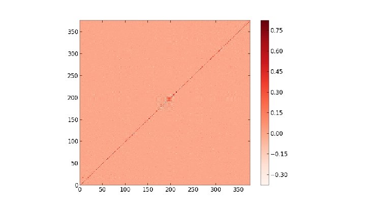
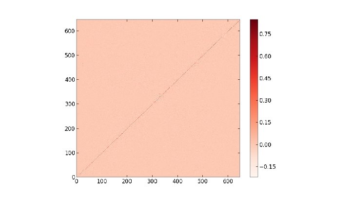
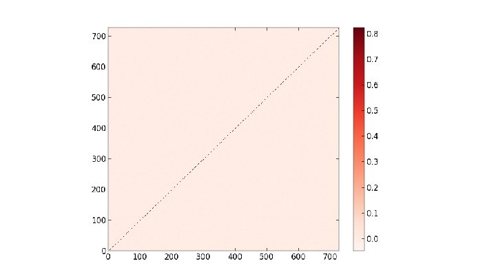
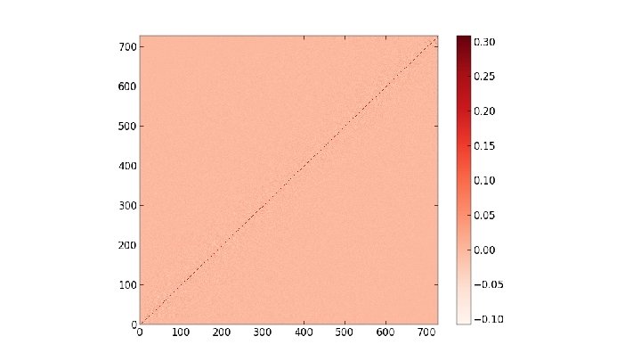
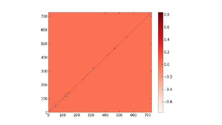
Heat Kernels of Max Clusters The main object of interest here is the heat kernel h(i, j, t) = Σk∈{0. . . |V|}e-λkt φki φkj where V is the graph's vertex set, and {λk} and {φk} are the eigenvalues and eigenvectors of the probabilistic graph laplacian matrix (respectively) computed using a max cluster percolated at some probability. Considering the diagonal h(i, i, t) as t evolves, we search for a power law by plotting t vs h(i, i, t) log-log. From there we can take the slopes of resulting straight line fits as the power law exponent. We also consider the full heat kernel h(x, y, t) as time increases

Power law behaviour: t vs h(x, x, t) for varied p (SG X SG)

Variation of these growth rates as p→ 1 As we vary p, how do these power law exponents behave? We address this by averaging all exponents (corresponding to each vertex in the cluster) On the two SG X SG graphs, they are going down (getting more negative) as p increases Generally they are a bit larger on the cell graph version On the Torus graph, they are going up (getting less negative)

Pictures of the full heat kernel h(x, y, t) at p =. 2 on SG X SG at t =. 25, 1. 75

Pictures of the full heat kernel h(x, y, t) at p =. 3 on SG X SG at t =. 25, 1. 75

Pictures of the full heat kernel h(x, y, t) at p =. 8 on SG X SG at t =. 25, 1. 75

Pictures of the full heat kernel h(x, y, t) at p = 1. 0 on SG X SG at t =. 25, 1. 75

Further exploration and final notes Proper interpretations of these data have been elusive We would like to be able to get better estimates of the critical probabilities Similarly, we’d like to identify where the transition from recurrent to transient occurs To this end we are currently analyzing the tendency of random walks to hit the graph boundaries Not all of our experiments have been performed on all of the fractals we have looked at