Oneway ANOVA Motivating Example Analysis of Variance Model

One-way ANOVA • • Motivating Example Analysis of Variance Model & Assumptions Data Estimates of the Model Analysis of Variance Multiple Comparisons Checking Assumptions One-way ANOVA Transformations

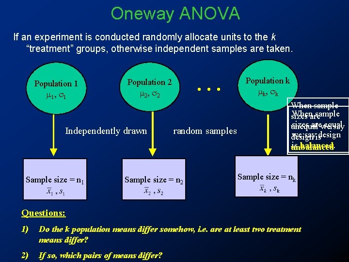
Oneway ANOVA If an experiment is conducted randomly allocate units to the k “treatment” groups, otherwise independent samples are taken. Population 1 m 1 , s 1 Independently drawn Sample size = n 1 . . . Population 2 m 2 , s 2 random samples Sample size = n 2 Population k m k , sk When sample Whenare sample sizes arewe equal unequal say we sayisdesign is balanced. unbalanced Sample size = nk Questions: 1) Do the k population means differ somehow, i. e. are at least two treatment means differ? 2) If so, which pairs of means differ?

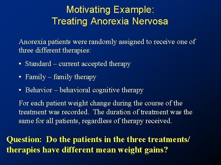
Motivating Example: Treating Anorexia Nervosa Anorexia patients were randomly assigned to receive one of three different therapies: • Standard – current accepted therapy • Family – family therapy • Behavior – behavioral cognitive therapy For each patient weight change during the course of the treatment was recorded. The duration of treatment was the same for all patients, regardless of therapy received. Question: Do the patients in the three treatments/ therapies have different mean weight gains?

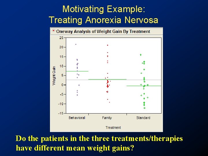
Motivating Example: Treating Anorexia Nervosa Do the patients in the three treatments/therapies have different mean weight gains?

Analysis of Variance • Analysis of Variance is a widely used statistical technique that partitions the total variability in our data into components of variability that are used to test hypotheses. • In One-way ANOVA, we wish to test the hypothesis: H 0 : 1 = 2 = = k against: HA : Not all population means are the same

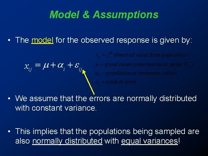
Model & Assumptions • The model for the observed response is given by: xij = + ij • We assume that the errors are normally distributed with constant variance. • This implies that the populations being sampled are also normally distributed with equal variances!

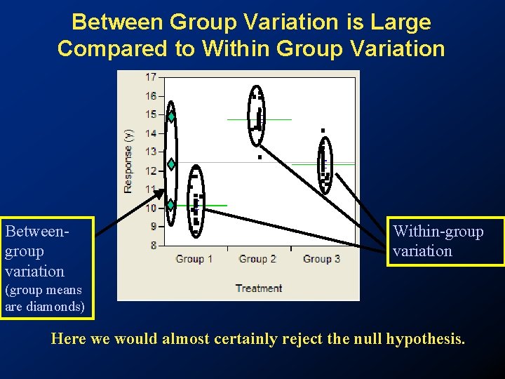
Analysis of Variance • In ANOVA, we compare the between-group variation with the within-group variation to assess whethere is a difference in the population means. • Thus by comparing these two measures of variance (spread) with one another, we are able to detect if there are true differences among the underlying group population means.

Analysis of Variance • If the variation between the sample means is large, relative to the variation within the samples, then we would be likely to detect significant differences among the sample means.

Between Group Variation is Large Compared to Within Group Variation Betweengroup variation Within-group variation (group means are diamonds) Here we would almost certainly reject the null hypothesis.

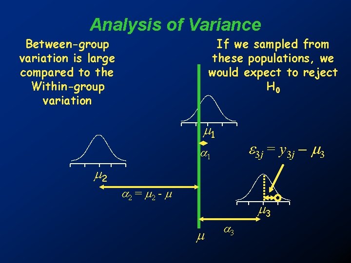
Analysis of Variance Between-group variation is large compared to the Within-group variation If we sampled from these populations, we would expect to reject H 0 1 3 j = y 3 j - 3 1 2 2 = 2 - 3 3

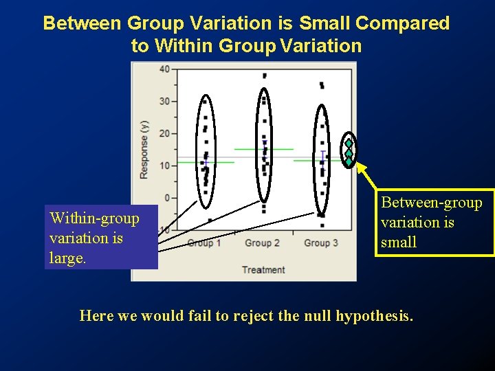
Analysis of Variance • If the variation between the sample means is small, relative to the variation within the samples, then there would be considerable overlap of observations in the different samples, and we would be unlikely to detect any differences among the population means.

Between Group Variation is Small Compared to Within Group Variation Within-group variation is large. Between-group variation is small Here we would fail to reject the null hypothesis.

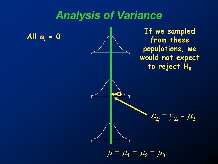
Analysis of Variance All i = 0 If we sampled from these populations, we would not expect to reject H 0 2 j = y 2 j - 2 = 1 = 2 = 3

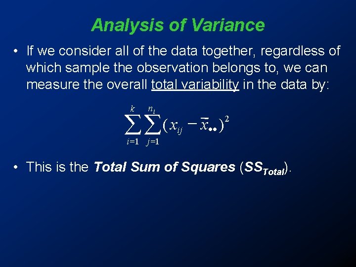
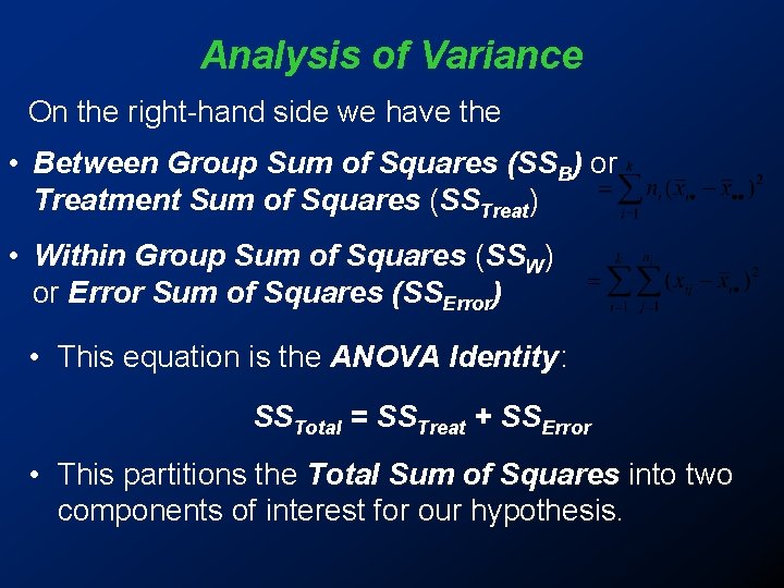
Analysis of Variance • If we consider all of the data together, regardless of which sample the observation belongs to, we can measure the overall total variability in the data by: k ni 2 åå ( xij x·· ) i =1 j =1 • This is the Total Sum of Squares (SSTotal).

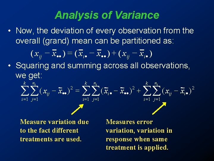
Analysis of Variance • Now, the deviation of every observation from the overall (grand) mean can be partitioned as: ( xij - x·· ) = ( xi· - x·· ) + ( xij - xi· ) • Squaring and summing across all observations, we get: k ni 2 2 2 = + ( x x ) åå ij ·· åå i· ·· åå ij i· i =1 j =1 Measure variation due to the fact different treatments are used. i =1 j =1 Measures error variation, variation in response when same treatment is applied.

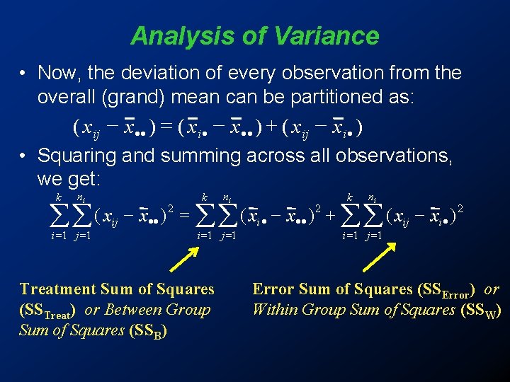
Analysis of Variance • Now, the deviation of every observation from the overall (grand) mean can be partitioned as: ( xij - x·· ) = ( xi· - x·· ) + ( xij - xi· ) • Squaring and summing across all observations, we get: k ni 2 2 2 = + ( x x ) åå ij ·· åå i· ·· åå ij i· i =1 j =1 Treatment Sum of Squares (SSTreat) or Between Group Sum of Squares (SSB) i =1 j =1 Error Sum of Squares (SSError) or Within Group Sum of Squares (SSW)

Analysis of Variance On the right-hand side we have the • Between Group Sum of Squares (SSB) or Treatment Sum of Squares (SSTreat) • Within Group Sum of Squares (SSW) or Error Sum of Squares (SSError) • This equation is the ANOVA Identity : SSTotal = SSTreat + SSError • This partitions the Total Sum of Squares into two components of interest for our hypothesis.

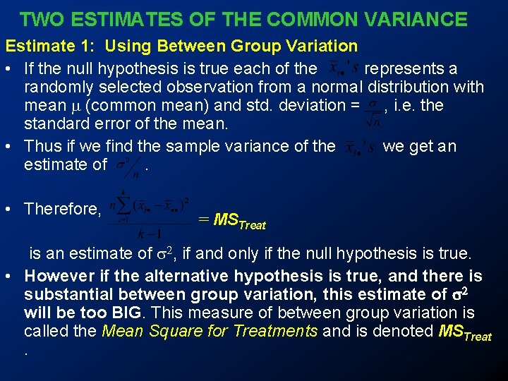
TWO ESTIMATES OF THE COMMON VARIANCE Estimate 1: Using Between Group Variation • If the null hypothesis is true each of the represents a randomly selected observation from a normal distribution with mean m (common mean) and std. deviation = , i. e. the standard error of the mean. • Thus if we find the sample variance of the we get an estimate of. • Therefore, = MSTreat is an estimate of s 2, if and only if the null hypothesis is true. • However if the alternative hypothesis is true, and there is substantial between group variation, this estimate of s 2 will be too BIG. This measure of between group variation is called the Mean Square for Treatments and is denoted MSTreat.

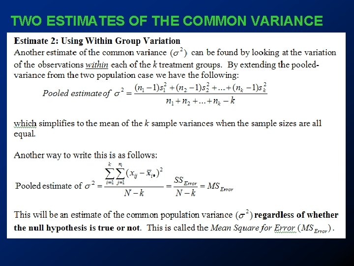
TWO ESTIMATES OF THE COMMON VARIANCE

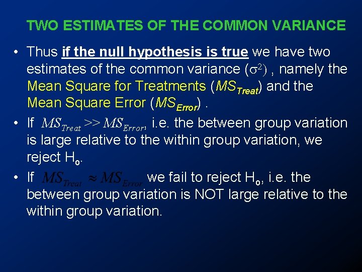
TWO ESTIMATES OF THE COMMON VARIANCE • Thus if the null hypothesis is true we have two estimates of the common variance (s 2) , namely the Mean Square for Treatments (MSTreat) and the Mean Square Error (MSError). • If MSTreat >> MSError, i. e. the between group variation is large relative to the within group variation, we reject Ho. • If we fail to reject H o, i. e. the between group variation is NOT large relative to the within group variation.

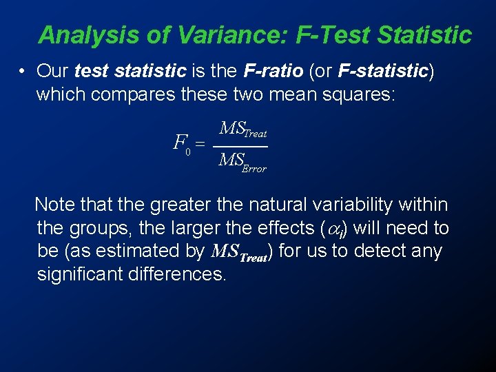
Analysis of Variance: F-Test Statistic • Our test statistic is the F-ratio (or F-statistic) which compares these two mean squares: F 0 = MSTreat MSError Note that the greater the natural variability within the groups, the larger the effects ( i) will need to be (as estimated by MSTreat) for us to detect any significant differences.

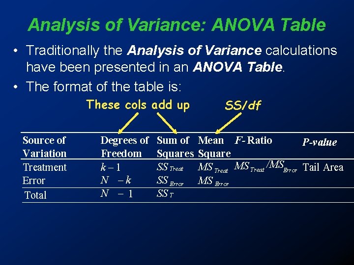
Analysis of Variance: ANOVA Table • Traditionally the Analysis of Variance calculations have been presented in an ANOVA Table. • The format of the table is: These cols add up Source of Variation Treatment Error Total Degrees of Freedom k– 1 N –k N – 1 Sum of Squares SS Treat SS Error SS T SS/df Mean F- Ratio P-value Square MS Treat /MSError Tail Area MS Error

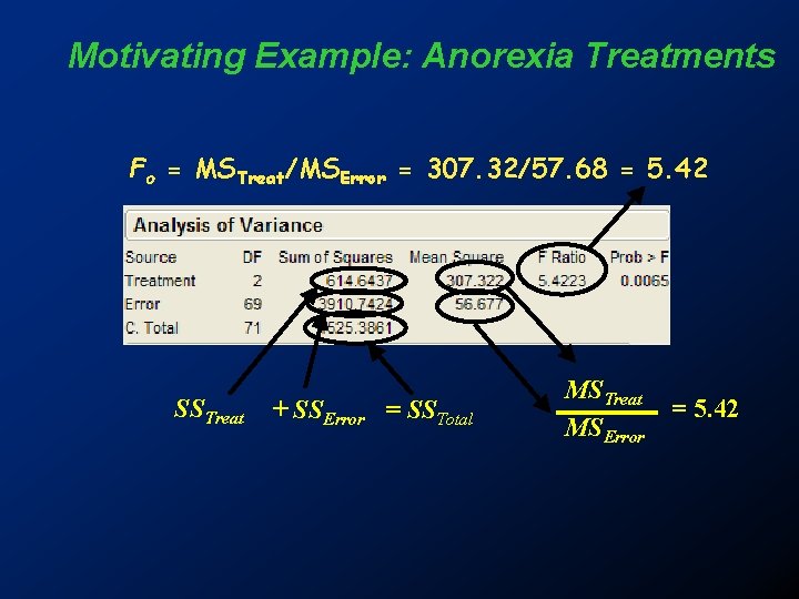
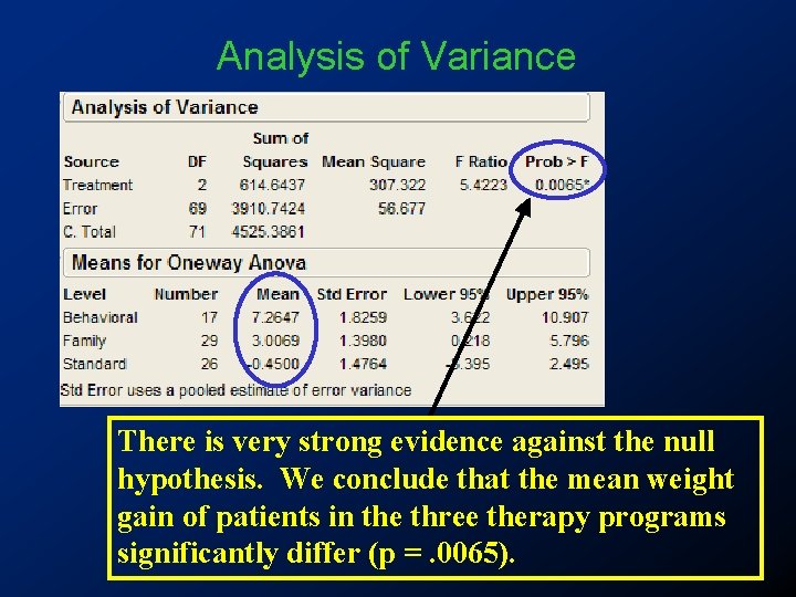
Motivating Example: Anorexia Treatments Fo = MSTreat/MSError = 307. 32/57. 68 = 5. 42 SSTreat + SSError = SSTotal MSTreat MSError = 5. 42

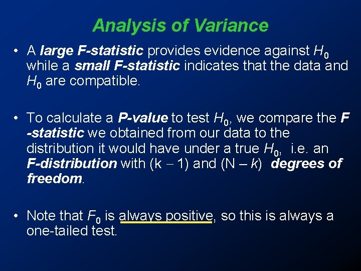
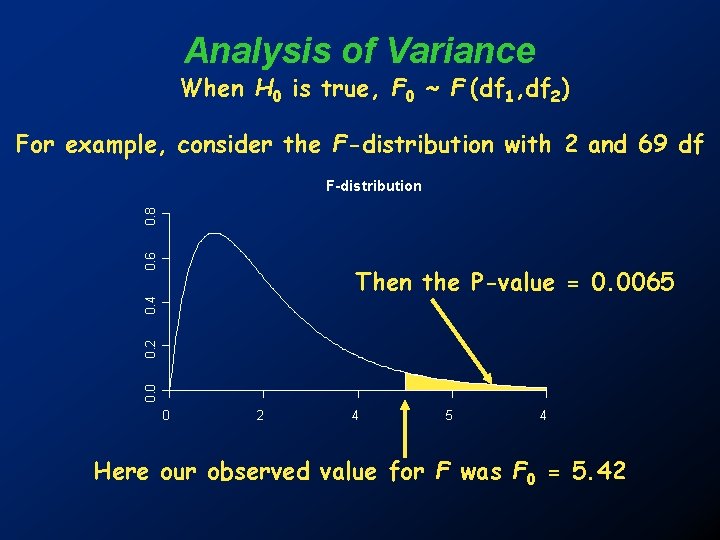
Analysis of Variance • A large F-statistic provides evidence against H 0 while a small F-statistic indicates that the data and H 0 are compatible. • To calculate a P-value to test H 0, we compare the F -statistic we obtained from our data to the distribution it would have under a true H 0, i. e. an F-distribution with (k - 1) and (N – k) degrees of freedom. • Note that F 0 is always positive, so this is always a one-tailed test.

Analysis of Variance When H 0 is true, F 0 ~ F (df 1, df 2) For example, consider the F-distribution with 2 and 69 df 0. 6 0. 8 F-distribution 0. 0 0. 2 0. 4 Then the P-value = 0. 0065 0 2 4 5 4 Here our observed value for F was F 0 = 5. 42

Analysis of Variance There is very strong evidence against the null hypothesis. We conclude that the mean weight gain of patients in the three therapy programs significantly differ (p =. 0065).

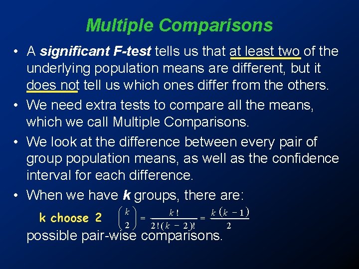
Multiple Comparisons • A significant F-test tells us that at least two of the underlying population means are different, but it does not tell us which ones differ from the others. • We need extra tests to compare all the means, which we call Multiple Comparisons. • We look at the difference between every pair of group population means, as well as the confidence interval for each difference. • When we have k groups, there are: k choose 2 æk ö k! k (k - 1 ) çç ÷÷ = = 2 ! ( k - 2 )! 2 è 2ø possible pair-wise comparisons.

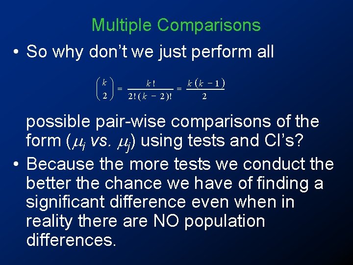
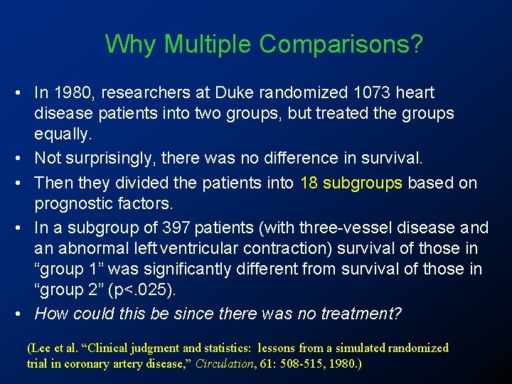
Multiple Comparisons • So why don’t we just perform all æk ö k! k (k - 1 ) çç ÷÷ = = 2 ! ( k - 2 )! 2 è 2ø possible pair-wise comparisons of the form ( i vs. j) using tests and CI’s? • Because the more tests we conduct the better the chance we have of finding a significant difference even when in reality there are NO population differences.

Why Multiple Comparisons? • In 1980, researchers at Duke randomized 1073 heart disease patients into two groups, but treated the groups equally. • Not surprisingly, there was no difference in survival. • Then they divided the patients into 18 subgroups based on prognostic factors. • In a subgroup of 397 patients (with three-vessel disease and an abnormal left ventricular contraction) survival of those in “group 1” was significantly different from survival of those in “group 2” (p<. 025). • How could this be since there was no treatment? (Lee et al. “Clinical judgment and statistics: lessons from a simulated randomized trial in coronary artery disease, ” Circulation, 61: 508 -515, 1980. )

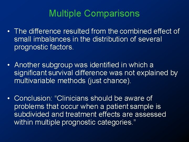
Multiple Comparisons • The difference resulted from the combined effect of small imbalances in the distribution of several prognostic factors. • Another subgroup was identified in which a significant survival difference was not explained by multivariable methods (just chance). • Conclusion: “Clinicians should be aware of problems that occur when a patient sample is subdivided and treatment effects are assessed within multiple prognostic categories. ”

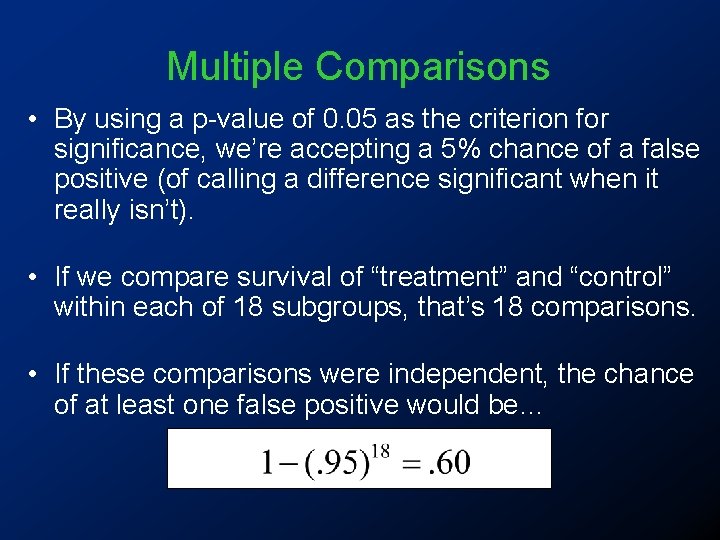
Multiple Comparisons • By using a p-value of 0. 05 as the criterion for significance, we’re accepting a 5% chance of a false positive (of calling a difference significant when it really isn’t). • If we compare survival of “treatment” and “control” within each of 18 subgroups, that’s 18 comparisons. • If these comparisons were independent, the chance of at least one false positive would be…

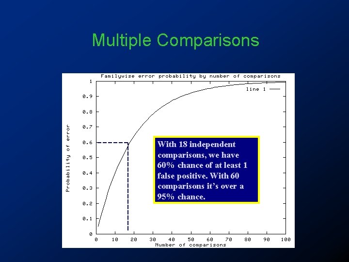
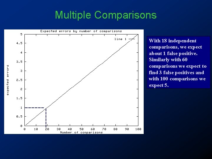
Multiple Comparisons With 18 independent comparisons, we have 60% chance of at least 1 false positive. With 60 comparisons it’s over a 95% chance.

Multiple Comparisons With 18 independent comparisons, we expect about 1 false positive. Similarly with 60 comparisons we expect to find 3 false positives and with 100 comparisons we expect 5.

Multiple Comparisons • If we estimate each comparison separately with 95% confidence, the overall error rate will be greater than 5%. • So, using ordinary pair-wise comparisons (i. e. lots of individual pooled t-tests), we tend to find too many significant differences between our sample means. • We need to modify our intervals so that they simultaneously contain the true differences with 95% confidence across the entire set of comparisons. • These modified intervals and tests are known as: simultaneous confidence methods OR multiple comparison procedures

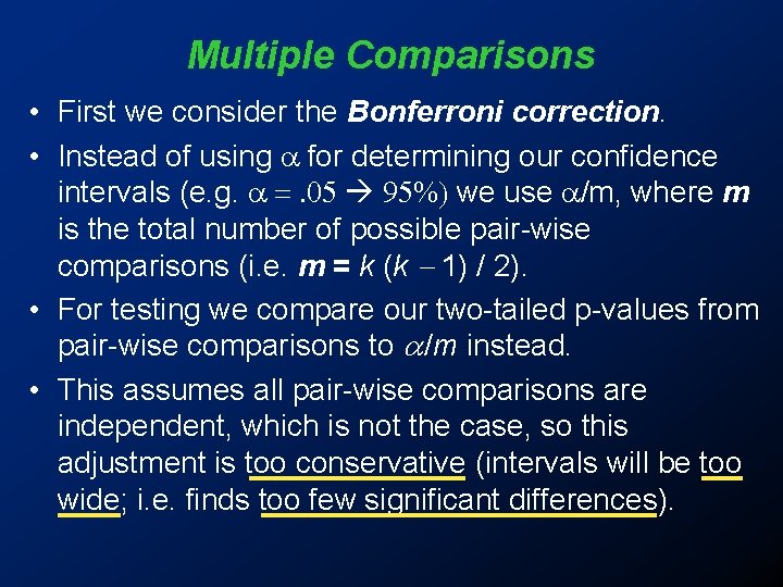
Multiple Comparisons • First we consider the Bonferroni correction. • Instead of using a for determining our confidence intervals (e. g. a =. 05 95%) we use a/m, where m is the total number of possible pair-wise comparisons (i. e. m = k (k - 1) / 2). • For testing we compare our two-tailed p-values from pair-wise comparisons to /m instead. • This assumes all pair-wise comparisons are independent, which is not the case, so this adjustment is too conservative (intervals will be too wide; i. e. finds too few significant differences).

Multiple Comparisons • As a better alternative we have Tukey Intervals. • The calculation of Tukey Intervals is quite complicated, but overcomes the problems of the unadjusted pair-wise comparisons finding too many significant differences (i. e. confidence intervals that are too narrow), and the Bonferroni correction finding too few significant differences (i. e. confidence intervals that are too wide). We will use Tukey Intervals and pair-wise tests

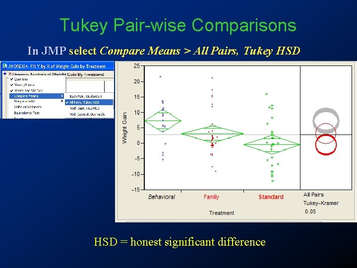
Tukey Pair-wise Comparisons In JMP select Compare Means > All Pairs, Tukey HSD = honest significant difference

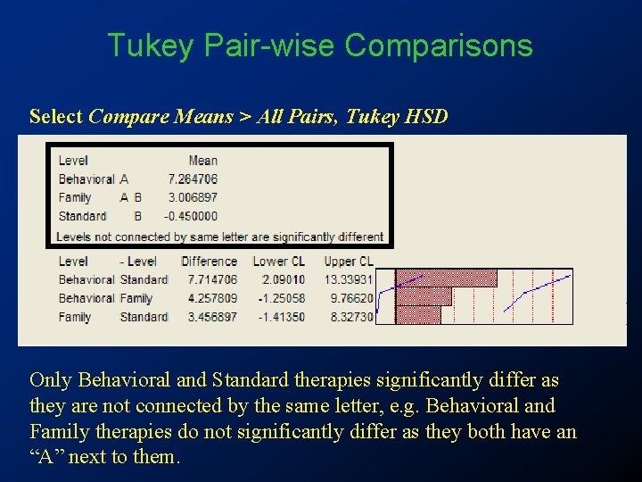
Tukey Pair-wise Comparisons Select Compare Means > All Pairs, Tukey HSD Only Behavioral and Standard therapies significantly differ as they are not connected by the same letter, e. g. Behavioral and Family therapies do not significantly differ as they both have an “A” next to them.

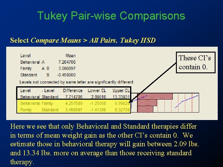
Tukey Pair-wise Comparisons Select Compare Means > All Pairs, Tukey HSD These CI’s contain 0. Here we see that only Behavioral and Standard therapies differ in terms of mean weight gain as the other CI’s contain 0. We estimate those in behavioral therapy will gain between 2. 09 lbs. and 13. 34 lbs. more on average than those receiving standard therapy.

Checking Assumptions: Independence • The observations within each sample must be independent of one another. This is determined by how the samples were taken or experiment was conducted. • Observational Studies: the random samples must be taken from independent populations. • Experimental Studies: the experimental units must be randomly allocated to treatment.

Checking Assumptions: Equality of Variance • Equality of variance is very important in One-way ANOVA. • We check equality of variance using Levene’s, Bartlett’s, Brown-Forsythe, or O’Brien’s Tests. • If the assumption of equal population variances is not satisfied (small P-value from these tests), we can try transforming the data or use Welch’s ANOVA which allows the variances to be unequal.

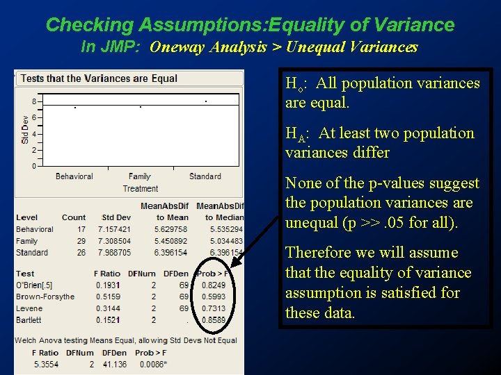
Checking Assumptions: Equality of Variance In JMP: Oneway Analysis > Unequal Variances Ho: All population variances are equal. HA: At least two population variances differ None of the p-values suggest the population variances are unequal (p >>. 05 for all). Therefore we will assume that the equality of variance assumption is satisfied for these data.

Checking Assumptions: Equality of Variance • For many data sets, we often find there is a relationship between the centre of the data and the spread of the data: • In particular, samples with low means (or medians) often have small spread while samples with large means (or medians) often have large spread (or vice versa). • The positive relationship between the mean and variance (or between the median and midspread) in different samples is often true for data that have right-skewed distributions.

Checking Assumptions: Equality of Variance • If the variance of the samples is increasing as the sample means increase a log or square root transformation is often times used. • However we can only use a log transformation if we wish to be able to back-transform and interpret our confidence intervals meaningfully (see later).

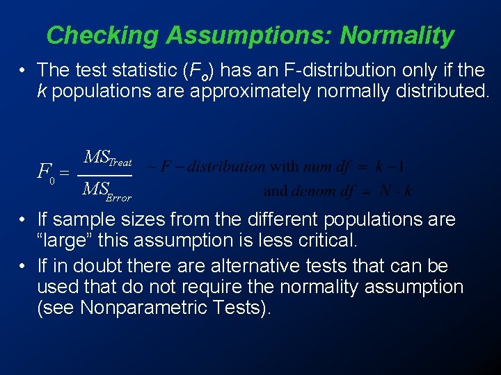
Checking Assumptions: Normality • The test statistic (Fo) has an F-distribution only if the k populations are approximately normally distributed. F 0 = MSTreat MSError • If sample sizes from the different populations are “large” this assumption is less critical. • If in doubt there alternative tests that can be used that do not require the normality assumption (see Nonparametric Tests).

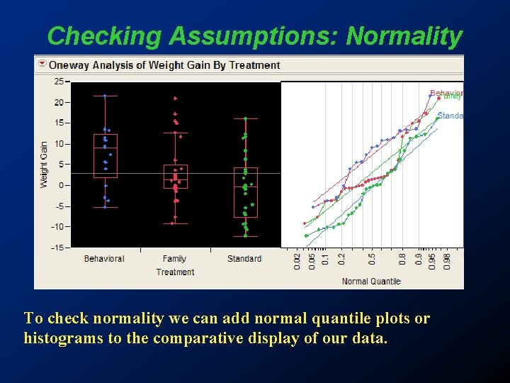
Checking Assumptions: Normality To check normality we can add normal quantile plots or histograms to the comparative display of our data.

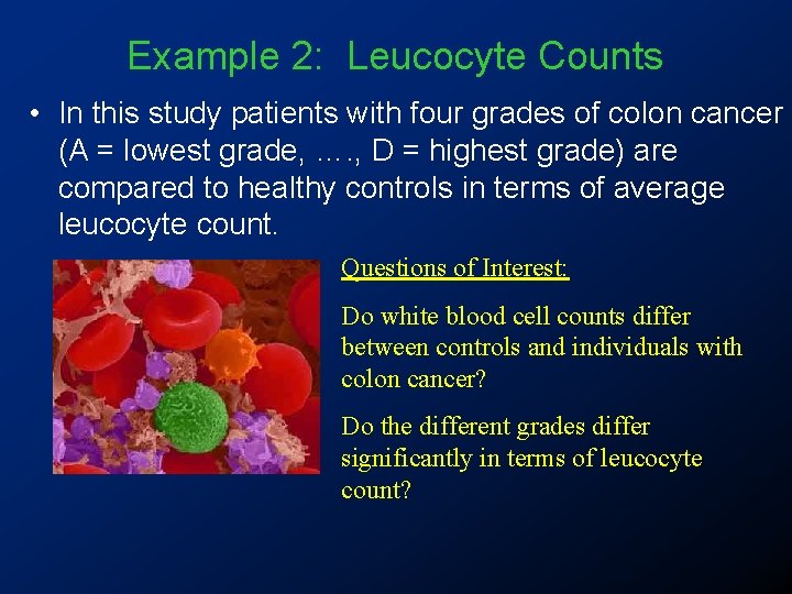
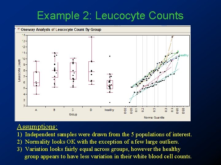
Example 2: Leucocyte Counts • In this study patients with four grades of colon cancer (A = lowest grade, …. , D = highest grade) are compared to healthy controls in terms of average leucocyte count. Questions of Interest: Do white blood cell counts differ between controls and individuals with colon cancer? Do the different grades differ significantly in terms of leucocyte count?

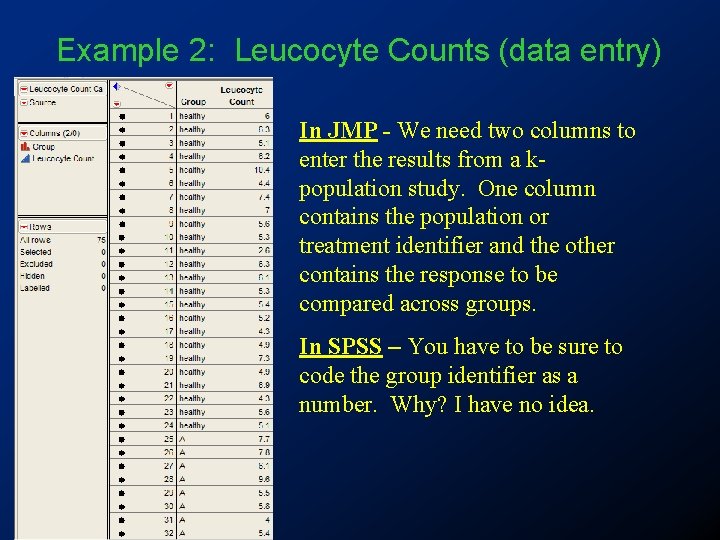
Example 2: Leucocyte Counts (data entry) In JMP - We need two columns to enter the results from a kpopulation study. One column contains the population or treatment identifier and the other contains the response to be compared across groups. In SPSS – You have to be sure to code the group identifier as a number. Why? I have no idea.

Example 2: Leucocyte Counts Assumptions: 1) Independent samples were drawn from the 5 populations of interest. 2) Normality looks OK with the exception of a few large outliers. 3) Variation looks fairly equal across groups, however the healthy group appears to have less variation in their white blood cell counts.

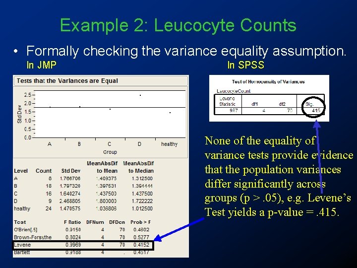
Example 2: Leucocyte Counts • Formally checking the variance equality assumption. In JMP In SPSS None of the equality of variance tests provide evidence that the population variances differ significantly across groups (p >. 05), e. g. Levene’s Test yields a p-value =. 415.

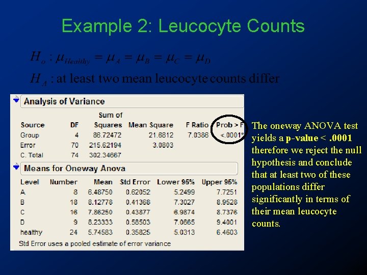
Example 2: Leucocyte Counts The oneway ANOVA test yields a p-value <. 0001 therefore we reject the null hypothesis and conclude that at least two of these populations differ significantly in terms of their mean leucocyte counts.

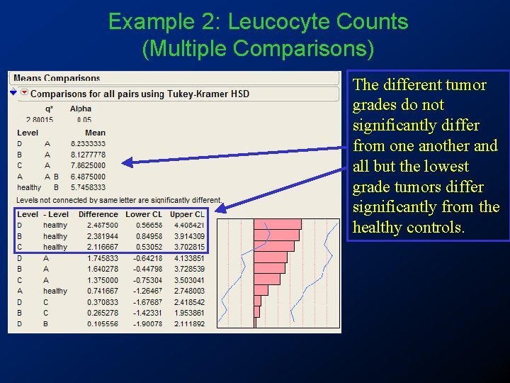
Example 2: Leucocyte Counts (Multiple Comparisons) The different tumor grades do not significantly differ from one another and all but the lowest grade tumors differ significantly from the healthy controls.

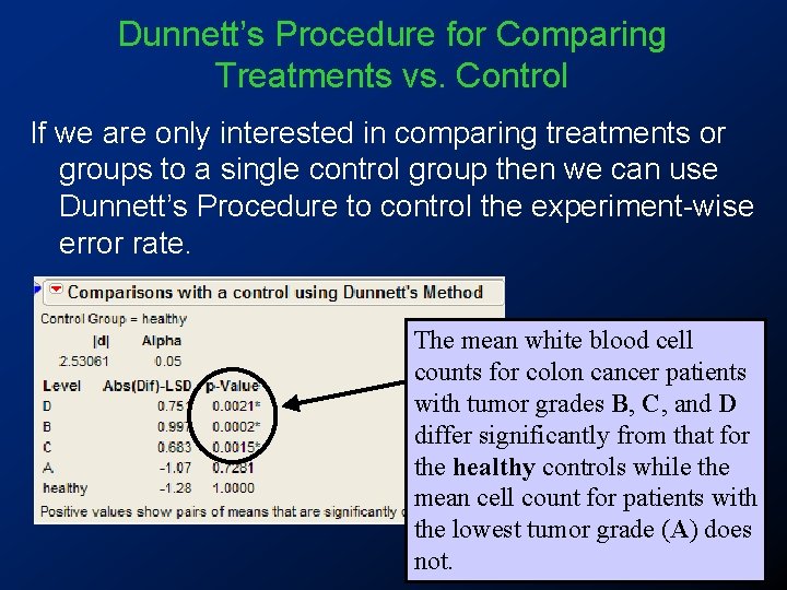
Dunnett’s Procedure for Comparing Treatments vs. Control If we are only interested in comparing treatments or groups to a single control group then we can use Dunnett’s Procedure to control the experiment-wise error rate. The mean white blood cell counts for colon cancer patients with tumor grades B, C, and D differ significantly from that for the healthy controls while the mean cell count for patients with the lowest tumor grade (A) does not.

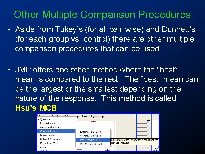
Other Multiple Comparison Procedures • Aside from Tukey’s (for all pair-wise) and Dunnett’s (for each group vs. control) there are other multiple comparison procedures that can be used. • JMP offers one other method where the “best” mean is compared to the rest. The “best” mean can be the largest or the smallest depending on the nature of the response. This method is called Hsu’s MCB.

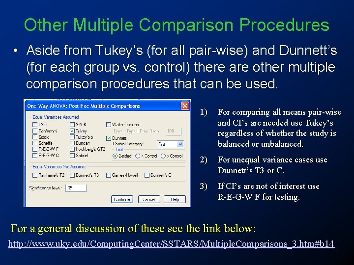
Other Multiple Comparison Procedures • Aside from Tukey’s (for all pair-wise) and Dunnett’s (for each group vs. control) there are other multiple comparison procedures that can be used. 1) For comparing all means pair-wise and CI’s are needed use Tukey’s regardless of whether the study is balanced or unbalanced. 2) For unequal variance cases use Dunnett’s T 3 or C. 3) If CI’s are not of interest use R-E-G-W F for testing. For a general discussion of these see the link below: http: //www. uky. edu/Computing. Center/SSTARS/Multiple. Comparisons_3. htm#b 14