OneWay Analysis of Variance ANOVA Aside l I

One-Way Analysis of Variance (ANOVA)

Aside l. I dislike the ANOVA chapter (11) in the book with a passion – if it were all written like this I wouldn’t use thing l Therefore, don’t worry if you don’t understand it, use my notes – Exam questions on ANOVA will come from my lectures and notes

One-Way ANOVA l One-Way Analysis of Variance ¡ aka One-Way ANOVA ¡ Most widely used statistical technique in all of statistics ¡ One-Way refers to the fact that only one IV and one DV are being analyzed (like the t-test) l i. e. An independent-samples t-test with treatment and control groups where the treatment (present in the tx grp and absent in the control grp) is the IV

One-Way ANOVA l Unlike the t-test, the ANOVA can look at levels or subgroups of IV’s ¡ ¡ The t-test can only test if an IV is there or not, not differences between subgroups of the IV I. e. our experiment is to test the effect of hair color (our IV) on intelligence l l One t-test can only test if brunettes are smarter than blondes, any other comparison would involve doing another t-test A one-way ANOVA can test many subgroups or levels of our IV “hair color”, for instance blondes, brunettes, and redheads are all subtypes of hair color, can so can be tested with one-way ANOVA

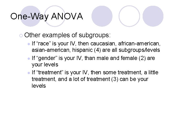
One-Way ANOVA ¡ Other examples of subgroups: If “race” is your IV, then caucasian, african-american, asian-american, hispanic (4) are all subgroups/levels l If “gender” is your IV, than male and female (2) are your levels l If “treatment” is your IV, then some treatment, a little treatment, and a lot of treatment (3) can be your levels l

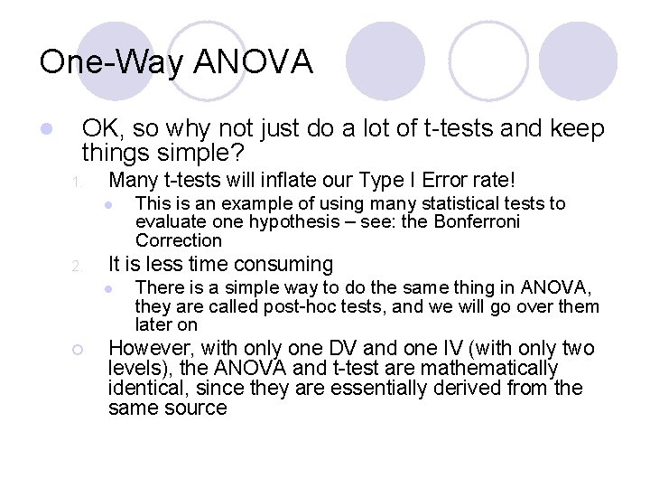
One-Way ANOVA l OK, so why not just do a lot of t-tests and keep things simple? 1. Many t-tests will inflate our Type I Error rate! l 2. It is less time consuming l ¡ This is an example of using many statistical tests to evaluate one hypothesis – see: the Bonferroni Correction There is a simple way to do the same thing in ANOVA, they are called post-hoc tests, and we will go over them later on However, with only one DV and one IV (with only two levels), the ANOVA and t-test are mathematically identical, since they are essentially derived from the same source

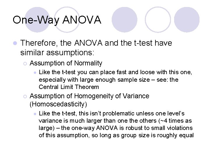
One-Way ANOVA l Therefore, the ANOVA and the t-test have similar assumptions: ¡ Assumption of Normality l ¡ Like the t-test you can place fast and loose with this one, especially with large enough sample size – see: the Central Limit Theorem Assumption of Homogeneity of Variance (Homoscedasticity) l Like the t-test, this isn’t problematic unless one level’s variance is much larger than one the others (~4 times as large) – the one-way ANOVA is robust to small violations of this assumption, so long as group size is roughly equal

One-Way ANOVA ¡ Independence l of Observations Like the t-test, the ANOVA is very sensitive to violations of this assumption – if violated it is more appropriate to use a Repeated-Measures ANOVA

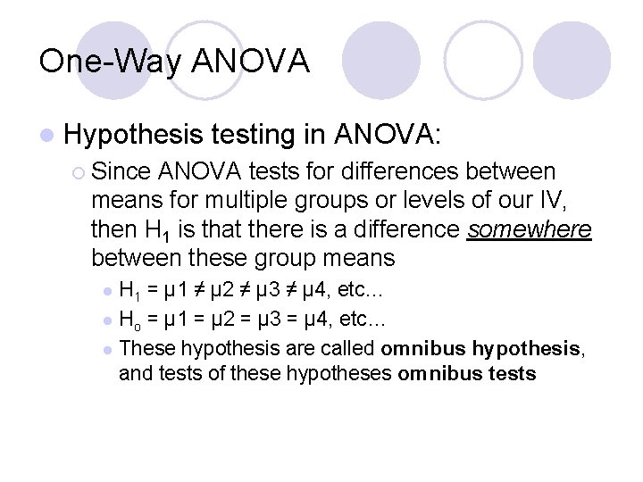
One-Way ANOVA l Hypothesis testing in ANOVA: ¡ Since ANOVA tests for differences between means for multiple groups or levels of our IV, then H 1 is that there is a difference somewhere between these group means H 1 = μ 1 ≠ μ 2 ≠ μ 3 ≠ μ 4, etc… l Ho = μ 1 = μ 2 = μ 3 = μ 4, etc… l These hypothesis are called omnibus hypothesis, and tests of these hypotheses omnibus tests l

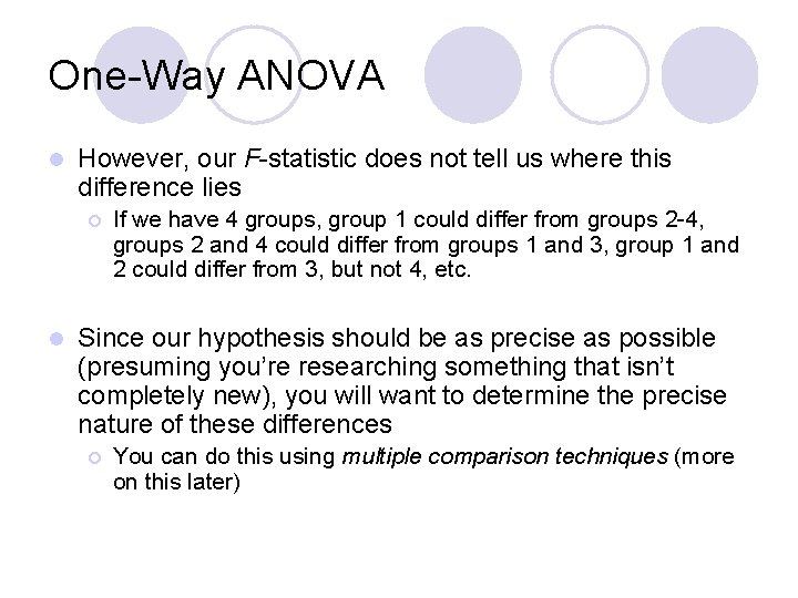
One-Way ANOVA l However, our F-statistic does not tell us where this difference lies ¡ l If we have 4 groups, group 1 could differ from groups 2 -4, groups 2 and 4 could differ from groups 1 and 3, group 1 and 2 could differ from 3, but not 4, etc. Since our hypothesis should be as precise as possible (presuming you’re researching something that isn’t completely new), you will want to determine the precise nature of these differences ¡ You can do this using multiple comparison techniques (more on this later)

One-Way ANOVA l The basic logic behind the ANOVA: ¡ The ANOVA yields and F-statistic (just like the ttest gave us a t-statistic) ¡ The basic form of the F-statistic is: MStreatment/MSerror ¡ MS = mean square or the mean of squares (why it is called this will be more obvious later)

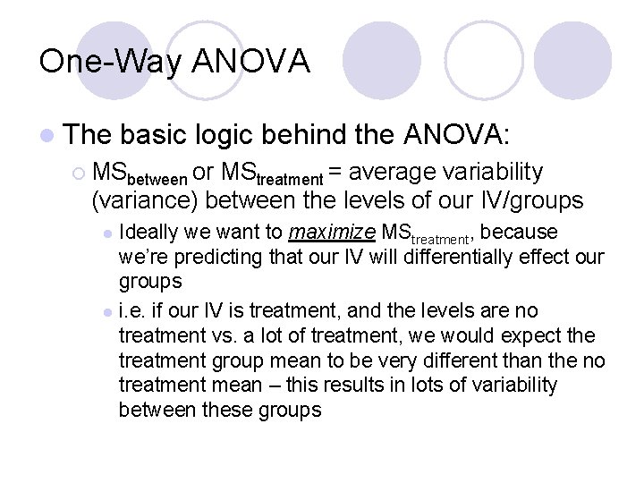
One-Way ANOVA l The basic logic behind the ANOVA: ¡ MSbetween or MStreatment = average variability (variance) between the levels of our IV/groups Ideally we want to maximize MStreatment, because we’re predicting that our IV will differentially effect our groups l i. e. if our IV is treatment, and the levels are no treatment vs. a lot of treatment, we would expect the treatment group mean to be very different than the no treatment mean – this results in lots of variability between these groups l

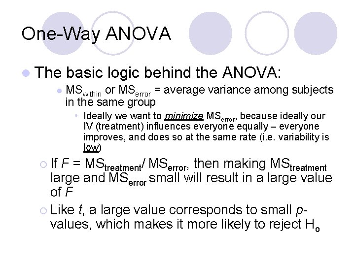
One-Way ANOVA l The l basic logic behind the ANOVA: MSwithin or MSerror = average variance among subjects in the same group • Ideally we want to minimize MSerror, because ideally our IV (treatment) influences everyone equally – everyone improves, and does so at the same rate (i. e. variability is low) ¡ If F = MStreatment/ MSerror, then making MStreatment large and MSerror small will result in a large value of F ¡ Like t, a large value corresponds to small pvalues, which makes it more likely to reject Ho

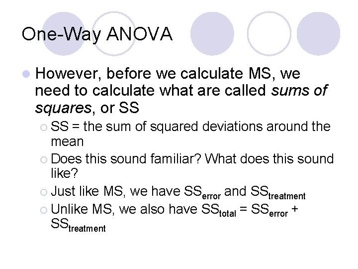
One-Way ANOVA l However, before we calculate MS, we need to calculate what are called sums of squares, or SS ¡ SS = the sum of squared deviations around the mean ¡ Does this sound familiar? What does this sound like? ¡ Just like MS, we have SSerror and SStreatment ¡ Unlike MS, we also have SStotal = SSerror + SStreatment

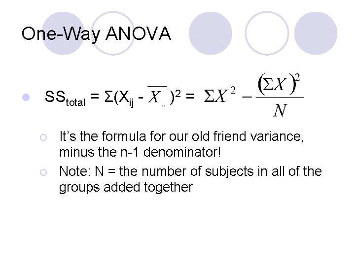
One-Way ANOVA l SStotal = Σ(Xij ¡ ¡ )2 = It’s the formula for our old friend variance, minus the n-1 denominator! Note: N = the number of subjects in all of the groups added together

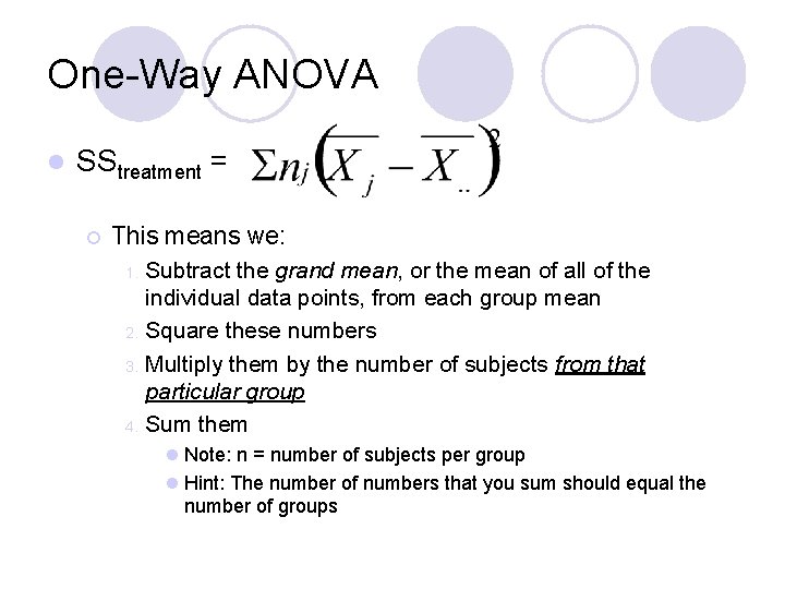
One-Way ANOVA l SStreatment = ¡ This means we: Subtract the grand mean, or the mean of all of the individual data points, from each group mean 2. Square these numbers 3. Multiply them by the number of subjects from that particular group 4. Sum them 1. l Note: n = number of subjects per group l Hint: The number of numbers that you sum should equal the number of groups

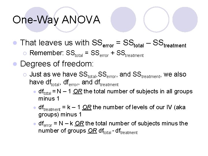
One-Way ANOVA l That leaves us with SSerror = SStotal – SStreatment ¡ l Remember: SStotal = SSerror + SStreatment Degrees of freedom: ¡ Just as we have SStotal, SSerror, and SStreatment, we also have dftotal, dferror, and dftreatment l l l dftotal = N – 1 OR the total number of subjects in all groups minus 1 dftreatment = k – 1 OR the number of levels of our IV (aka groups) minus 1 dferror = N – k OR the total number of subjects minus the number of groups OR dftotal - dftreatment

One-Way ANOVA l Now that we have our SS and df, we can calculate MS ¡ MStreatment = SStreatment/dftreatment ¡ MSerror = SSerror/dferror l Remember: ¡ MSbetween or MStreatment = average variability (variance) between the levels of our IV/groups ¡ MSwithin or MSerror = average variance among subjects in the same group

One-Way ANOVA l We then use this to calculate our Fstatistic: ¡F = MStreatment/ MSerror l The p-value associated with this F-statistic is a function of both F and your df ¡ Higher F and/or df Lower p ¡ Recall: df = n & # levels of your IV l More S’s and/or fewer levels Higher df Lower p

One-Way ANOVA l How can we change our experiment to increase the likelihood of a significant result/decrease p? ¡ Larger ES Higher F: l ¡ Increase the potency of the IV Higher df l l More S’s Fewer # levels of your IV • Collapse across groups – Instead of looking at Kids vs. Young Adults vs. Adults, look at Children vs. Adults only • Worst way to decrease p as this sacrifices how subtle-ly you can test your theory

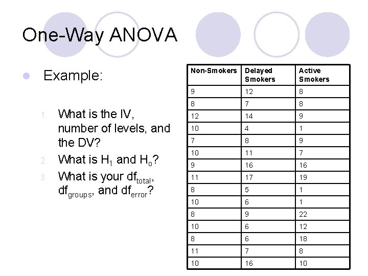
One-Way ANOVA l Example: ¡ What effect does smoking have on performance? Spilich, June, and Renner (1992) asked nonsmokers (NS), smokers who had delayed smoking for three hours (DS), and smokers who were actively smoking (AS) to perform a pattern recognition task in which they had to locate a target on a screen. The data follow:

One-Way ANOVA l Example: 1. 2. 3. What is the IV, number of levels, and the DV? What is H 1 and Ho? What is your dftotal, dfgroups, and dferror? Non-Smokers Delayed Smokers Active Smokers 9 12 8 8 7 8 12 14 9 10 4 1 7 8 9 10 11 7 9 16 16 11 17 19 8 5 1 10 6 1 8 9 22 10 6 12 8 6 18 11 7 8 10 16 10

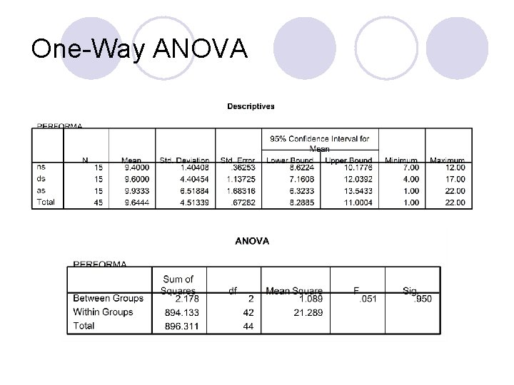
One-Way ANOVA

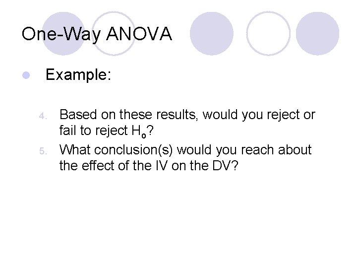
One-Way ANOVA l Example: 4. 5. Based on these results, would you reject or fail to reject Ho? What conclusion(s) would you reach about the effect of the IV on the DV?

One-Way ANOVA l Assumptions of ANOVA: ¡ Independence of Observations ¡ Homoscedasticity ¡ Normality l Equal sample sizes – not technically an assumption, but effects the other 3 l How do we know if we violate one (or more) of these? What do we do?

One-Way ANOVA l Independence of Observations ¡ Identified methodologically ¡ Other than using repeated-measures tests (covered later), nothing you can do l Equal ¡ Add Sample Sizes more S’s to the smaller group ¡ DON’T delete S’s from the larger one

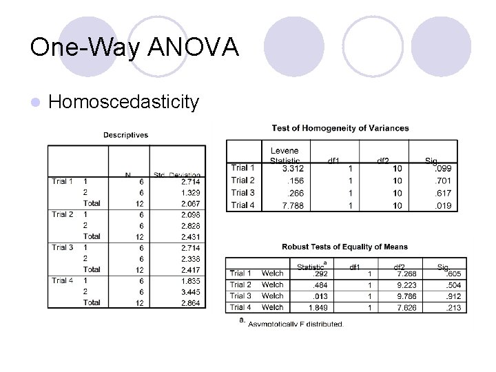
One-Way ANOVA l Homoscedasticity ¡ Identified using Levene’s Test or the Welch Procedure ¡ Again, don’t sweat the book, SPSS will do it for you ¡ If detected (and group sizes very unequal), use appropriate transformation

One-Way ANOVA l Homoscedasticity

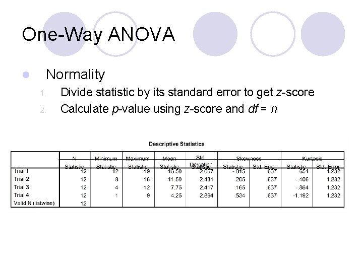
One-Way ANOVA l Normality ¡ Can identify with histograms of DV’s (IV’s are supposed to be non-normal) ¡ More appropriate to use skewness and kurtosis statistics ¡ If detected (and sample size very small), use appropriate transformation

One-Way ANOVA l Normality 1. 2. Divide statistic by its standard error to get z-score Calculate p-value using z-score and df = n

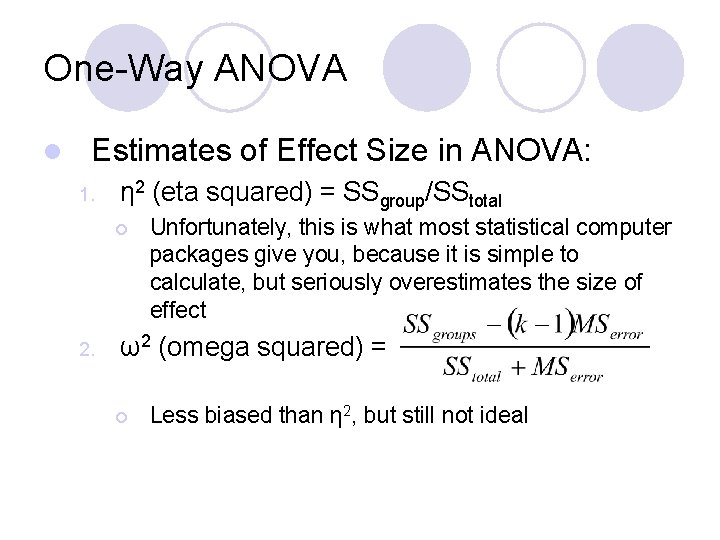
One-Way ANOVA l Estimates of Effect Size in ANOVA: 1. η 2 (eta squared) = SSgroup/SStotal ¡ 2. Unfortunately, this is what most statistical computer packages give you, because it is simple to calculate, but seriously overestimates the size of effect ω2 (omega squared) = ¡ Less biased than η 2, but still not ideal

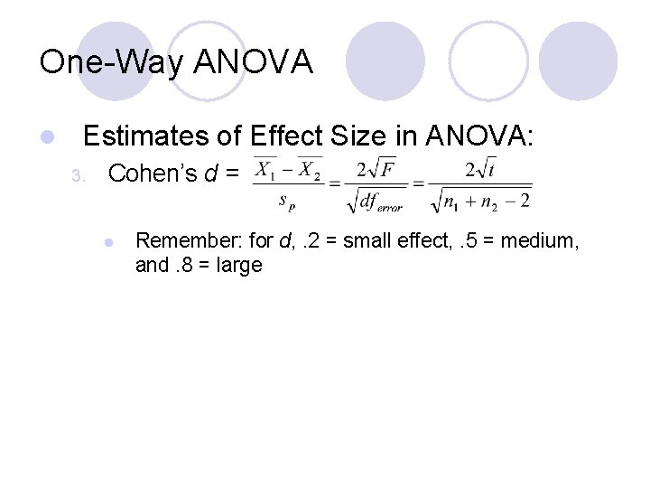
One-Way ANOVA l Estimates of Effect Size in ANOVA: 3. Cohen’s d = l Remember: for d, . 2 = small effect, . 5 = medium, and. 8 = large

One-Way ANOVA l Multiple Comparison Techniques: ¡ Remember: ANOVA tests for differences somewhere between group means, but doesn’t say where H 1 = μ 1 ≠ μ 2 ≠ μ 3 ≠ μ 4, etc… l If significant, group 1 could be different from groups 2 -4, groups 2 & 3 could be different from groups 1 and 4, etc. l Multiple comparison techniques attempt to detect specifically where these differences lie l

Multiple Comparison Techniques ¡ You could always run 2 -sample t-tests on all possible 2 -group combinations of your groups, although with our 4 group example this is 6 different tests ¡ Running 6 tests @ (α =. 05) = (α =. 05 x 6 =. 3) ¡ This would inflate what is called the familywise error rate – in our previous example, all of the 6 tests that we run are considered a family of tests, and the familywise error rate is the α for all 6 tests combined (. 3) – however, we want to keep this at. 05

Multiple Comparison Techniques ¡ To perform multiple comparisons with a significant omnibus F, or not to … ¡ Why would you look for a difference between two or more groups when your F said there isn’t one?

Multiple Comparison Techniques ¡ Some say this is what is called statistical fishing and is very bad – you should not be conducting statistical tests willy-nilly without just cause or a theoretical reason for doing so ¡Think of someone fishing in a lake, you don’t know if anything is there, but you’ll keep trying until you find something – the idea is that if your hypothesis is true, you shouldn’t have to look to hard to find it, because if you look for anything hard enough you tend to find it

Multiple Comparison Techniques ¡ However, others would say that the omnibus test is underpowered, particularly with a large number of groups and if only a few significant differences are predicted among them i. e. H 1 = μ 1 ≠ μ 2 ≠ μ 3 ≠ μ 4 … μ 10 l If you only predict groups 1 and 5 will differ, you are unlikely to get a significant omnibus F unless you have a ton of S’s l I and most statisticians fall on this side of the argument – i. e. it’s OK to ignore the omnibus test if you have a theoretical reason to predict specific differences among groups l

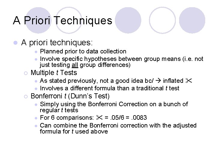
A Priori Techniques l A priori techniques: l l ¡ Multiple t Tests l l ¡ Planned prior to data collection Involve specific hypotheses between group means (i. e. not just testing all group differences) As stated previously, not a good idea bc/ inflated Involves a different formula than a traditional t test Bonferroni t (Dunn’s Test) l l l Simply using the Bonferroni Correction on a bunch of regular t tests For 6 comparisons: =. 05/6 =. 0083 Can combine the Bonferroni correction with the adjusted formula for t used above

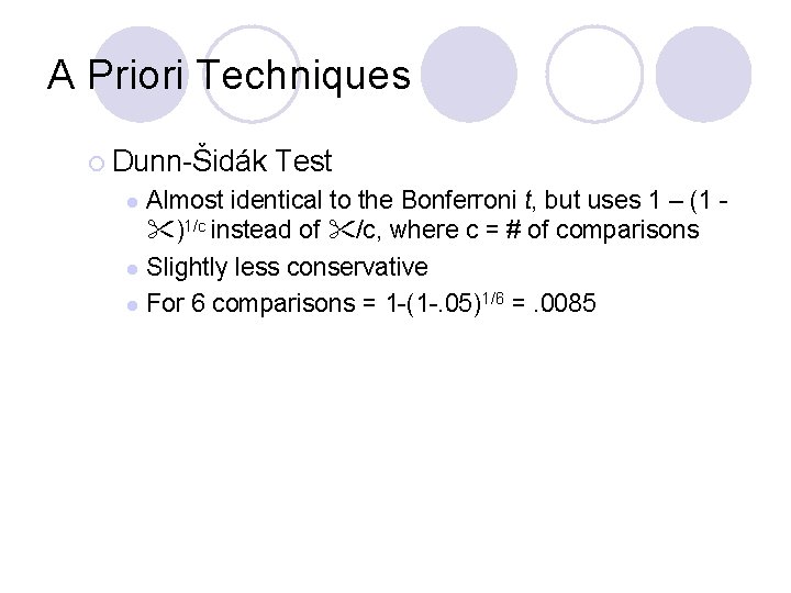
A Priori Techniques ¡ Dunn-Šidák Test Almost identical to the Bonferroni t, but uses 1 – (1 )1/c instead of /c, where c = # of comparisons l Slightly less conservative l For 6 comparisons = 1 -(1 -. 05)1/6 =. 0085 l

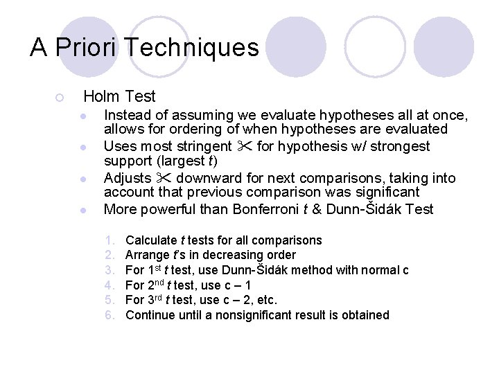
A Priori Techniques ¡ Holm Test l l Instead of assuming we evaluate hypotheses all at once, allows for ordering of when hypotheses are evaluated Uses most stringent for hypothesis w/ strongest support (largest t) Adjusts downward for next comparisons, taking into account that previous comparison was significant More powerful than Bonferroni t & Dunn-Šidák Test 1. 2. 3. 4. 5. 6. Calculate t tests for all comparisons Arrange t’s in decreasing order For 1 st t test, use Dunn-Šidák method with normal c For 2 nd t test, use c – 1 For 3 rd t test, use c – 2, etc. Continue until a nonsignificant result is obtained

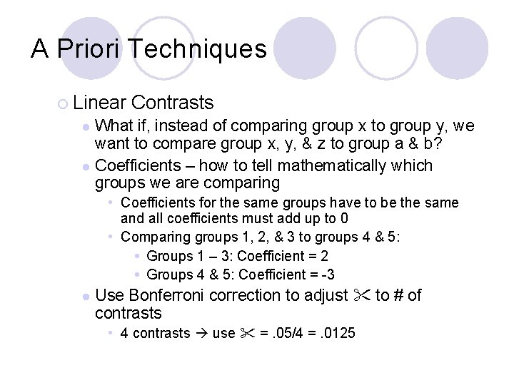
A Priori Techniques ¡ Linear Contrasts What if, instead of comparing group x to group y, we want to compare group x, y, & z to group a & b? l Coefficients – how to tell mathematically which groups we are comparing l • Coefficients for the same groups have to be the same and all coefficients must add up to 0 • Comparing groups 1, 2, & 3 to groups 4 & 5: Groups 1 – 3: Coefficient = 2 Groups 4 & 5: Coefficient = -3 l Use Bonferroni correction to adjust to # of contrasts • 4 contrasts use =. 05/4 =. 0125

A Priori Techniques ¡ Orthogonal Contrasts What if you want to compare groups within a contrast? l I. e. Group 1 vs. Groups 2 & 3 and Group 2 vs. Group 3 l Assigning coefficients is the same, but calculations are different (don’t worry about how different, just focus on the linear vs. orthogonal difference) l

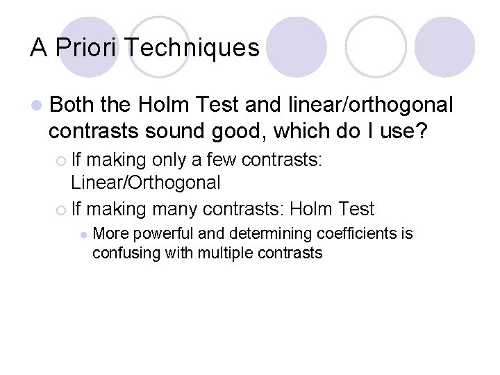
A Priori Techniques l Both the Holm Test and linear/orthogonal contrasts sound good, which do I use? ¡ If making only a few contrasts: Linear/Orthogonal ¡ If making many contrasts: Holm Test l More powerful and determining coefficients is confusing with multiple contrasts

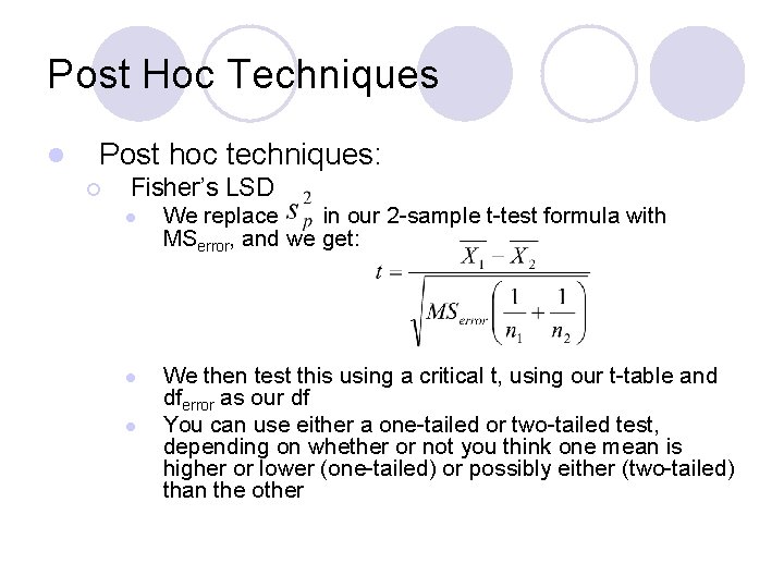
Post Hoc Techniques l Post hoc techniques: ¡ Fisher’s LSD l We replace in our 2 -sample t-test formula with MSerror, and we get: l We then test this using a critical t, using our t-table and dferror as our df You can use either a one-tailed or two-tailed test, depending on whether or not you think one mean is higher or lower (one-tailed) or possibly either (two-tailed) than the other l

Post Hoc Techniques ¡ Fisher’s LSD l l l ¡ However, with more than 3 groups, using Fisher’s LSD results in an inflation of (i. e. with 4 groups α =. 1) You could use the Bonferroni method to correct for this, but then why not just use it in the first place? This is why Fisher’s LSD is no longer widely used and other methods are preferred Newman-Keuls Test l l Like Fisher’s LSD, allows the familywise >. 05 Pretty crappy test for that reason

Post Hoc Techniques ¡ Scheffé’s Test l l ¡ Fishers LSD & Neuman-Keuls = not conservative enough = too easy to find significant results Scheffé’s Test = too conservative = result in a low degree of Type I Error but too high Type II Error (incorrectly rejects H 1) = too hard to find significant results Tukey’s Honestly Significant Difference (HSD) test l Very popular, but conservative

Post Hoc Techniques ¡ Ryan/Einot/Gabriel/Welsch (REGWQ) Procedure Like Tukey’s HSD, but adjusts (like the DunnŠidák Test) to make the test less conservative l Good compromise of Type I/Type II Error l ¡ Dunnett’s Test Specifically designed for comparing a control group with several treatment groups l Most powerful test in this case l

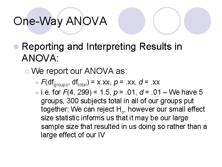
One-Way ANOVA l Reporting and Interpreting Results in ANOVA: ¡ We report our ANOVA as: F(dfgroups, dftotal) = x. xx, p =. xx, d =. xx l i. e. for F(4, 299) = 1. 5, p =. 01, d =. 01 – We have 5 groups, 300 subjects total in all of our groups put together; We can reject Ho, however our small effect size statistic informs us that it may be our large sample size that resulted in us doing so rather than a large effect of our IV l