Network Tomography and Anomaly Detection Mark Coates Tarem

Network Tomography and Anomaly Detection Mark Coates Tarem Ahmed Network map from www. opte. org

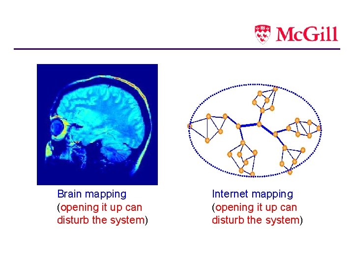
Brain mapping (opening it up can disturb the system) Internet mapping (opening it up can disturb the system)

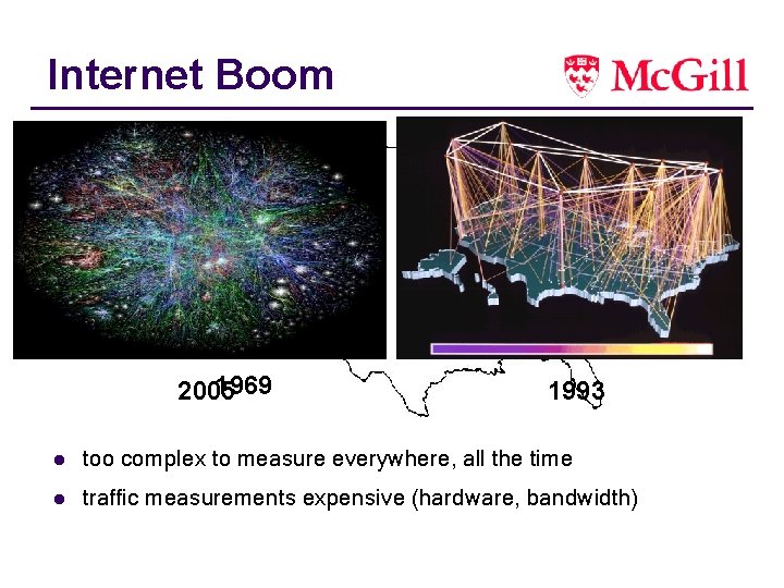
Internet Boom 1969 2005 1993 l too complex to measure everywhere, all the time l traffic measurements expensive (hardware, bandwidth)

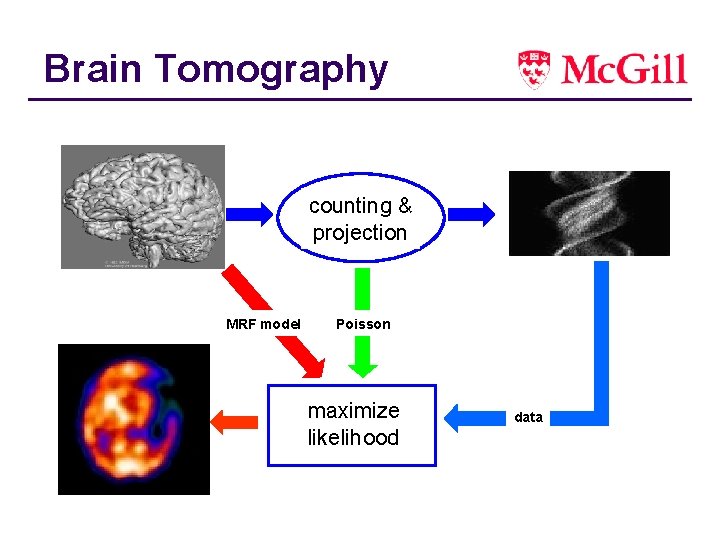
Brain Tomography unknown object statistical& counting projection model prior knowledge MRF model Maximum likelihood estimate measurements physics Poisson maximize likelihood data

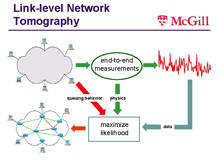
Link-level Network Tomography unknown object end-to-end measurements queuing prior knowledge behavior Maximum likelihood estimate measurements physics maximize likelihood data

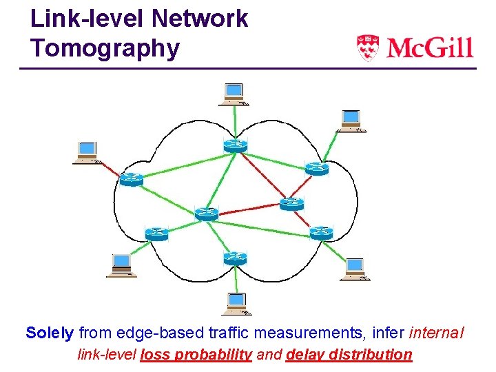
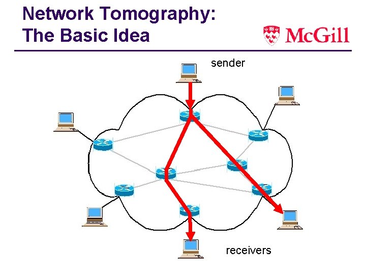
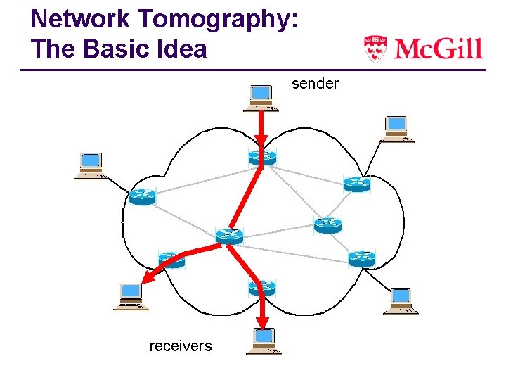
Link-level Network Tomography Solely from edge-based traffic measurements, infer internal link-level losstopology probability and delay distribution / connectivity

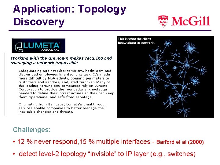
Application: Topology Discovery Challenges: • 12 % never respond, 15 % multiple interfaces - Barford et al (2000) • detect level-2 topology “invisible” to IP layer (e. g. , switches)

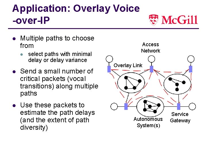
Application: Overlay Voice -over-IP l Multiple paths to choose from l select paths with minimal delay or delay variance l Send a small number of critical packets (vocal transitions) along multiple paths l Use these packets to estimate the path delays (and the extent of path diversity) Access Network Overlay Link Autonomous System(s) Service Gateway

Network Monitoring l Challenges l l Restricted measurement High volumes and high rates of data (sampling of traffic on Gb/s routers) High dimensional data (source/destination IP addresses, port numbers) Goals l l l Supply networking protocols with relevant performance information. Identify anomalous behaviour and operational transitions. Provide network administrators with appropriate notification or visualization.

Outline l Inference about network performance based on passive measurements or active probing l Two components to the talk: l l l Network tomography Network anomaly detection Focus on online, sequential approaches l l Account for non-stationary behaviour Don’t repeat work that has already been done

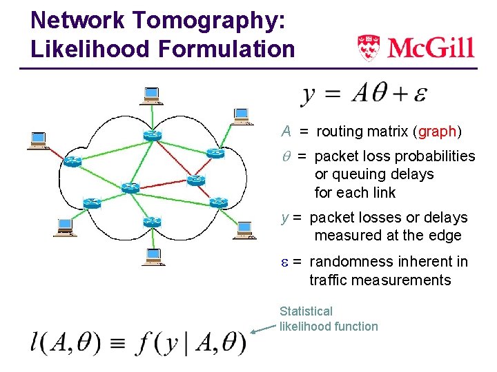
Network Tomography: Likelihood Formulation A = routing matrix (graph) = packet loss probabilities or queuing delays for each link y = packet losses or delays measured at the edge = randomness inherent in traffic measurements Statistical likelihood function

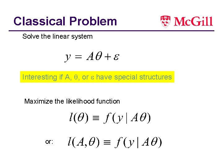
Classical Problem Solve the linear system Interesting if A, , or have special structures Maximize the likelihood function or:

Network Tomography: The Basic Idea sender receivers

Network Tomography: The Basic Idea sender receivers

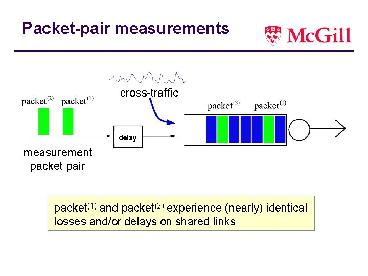
Packet-pair measurements cross-traffic delay measurement packet pair packet(1) and packet(2) experience (nearly) identical losses and/or delays on shared links

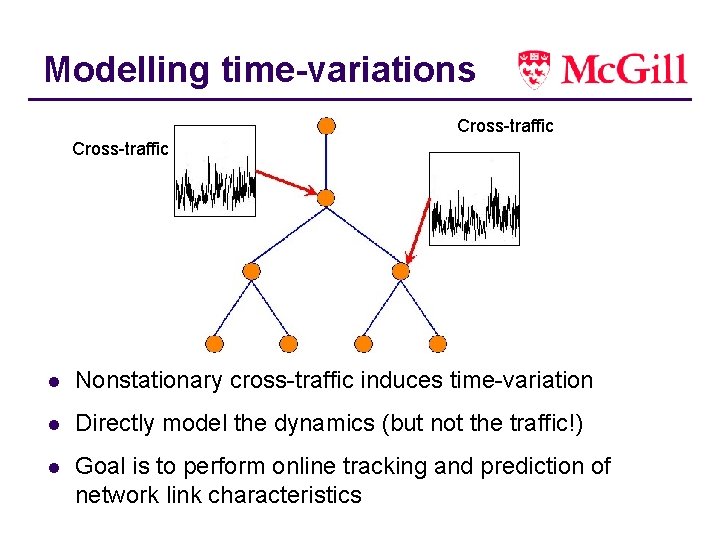
Modelling time-variations Cross-traffic l Nonstationary cross-traffic induces time-variation l Directly model the dynamics (but not the traffic!) l Goal is to perform online tracking and prediction of network link characteristics

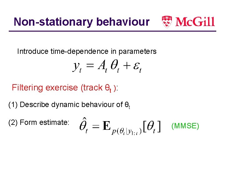
Non-stationary behaviour Introduce time-dependence in parameters Filtering exercise (track θt ): (1) Describe dynamic behaviour of θt (2) Form estimate: (MMSE)

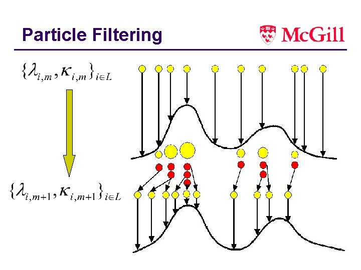
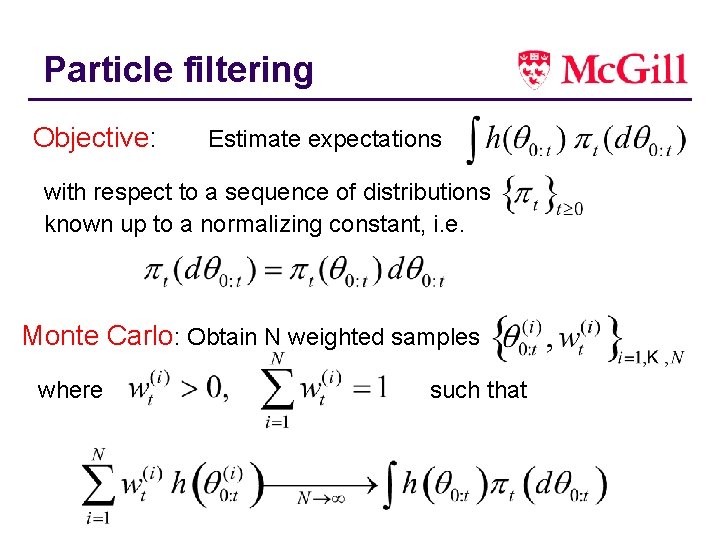
Particle Filtering

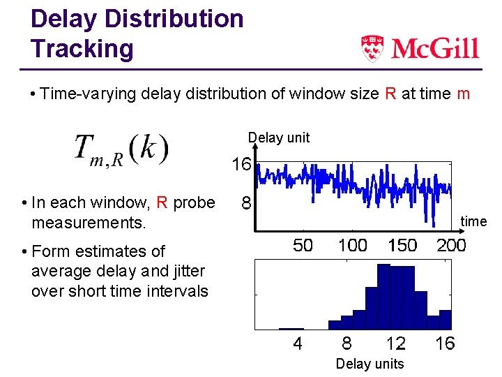
Delay Distribution Tracking • Time-varying delay distribution of window size R at time m Delay unit • In each window, R probe measurements. time • Form estimates of average delay and jitter over short time intervals Delay units

Dynamic Model • Queue/traffic model: 4 4 reflected random walk on [0, max_del] Probability Delay units

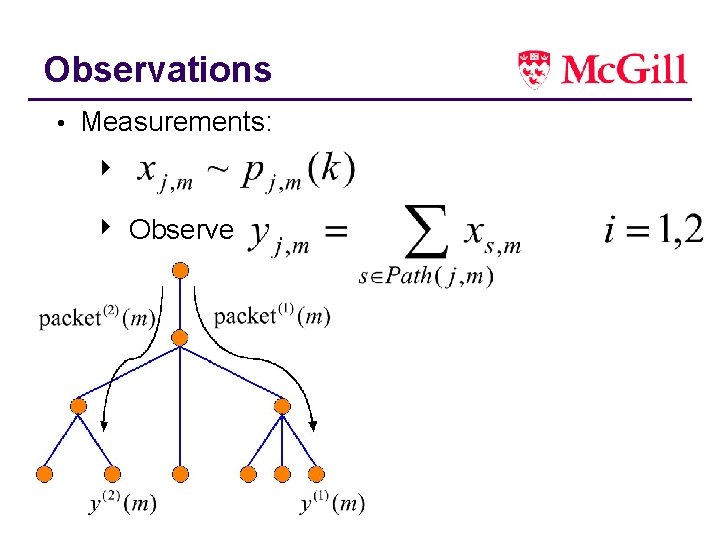
Observations • Measurements: 4 4 Observe

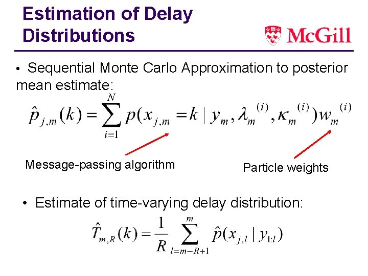
Estimation of Delay Distributions • Sequential Monte Carlo Approximation to posterior mean estimate: Message-passing algorithm Particle weights • Estimate of time-varying delay distribution:

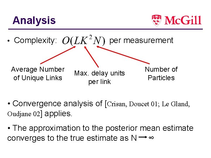
Analysis • Complexity: Average Number of Unique Links per measurement Max. delay units per link Number of Particles • Convergence analysis of [Crisan, Doucet 01; Le Gland, Oudjane 02] applies. • The approximation to the posterior mean estimate converges to the true estimate as N ∞

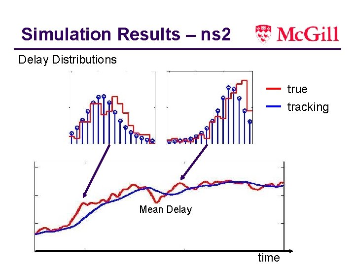
Simulation Results – ns 2 Delay Distributions true tracking Mean Delay time

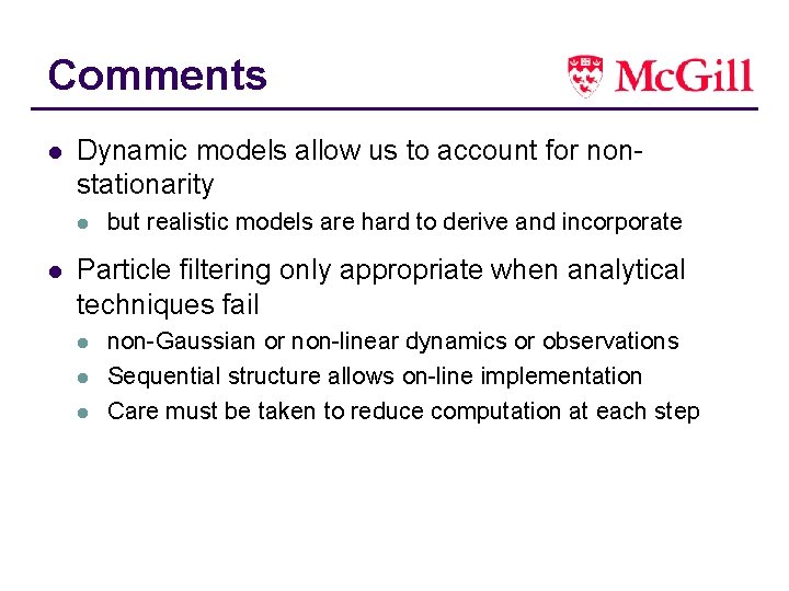
Comments l Dynamic models allow us to account for nonstationarity l l but realistic models are hard to derive and incorporate Particle filtering only appropriate when analytical techniques fail l non-Gaussian or non-linear dynamics or observations Sequential structure allows on-line implementation Care must be taken to reduce computation at each step

Network Anomaly Detection l In tomography, a primary challenge is the restriction on available measurements. l Anomaly detection – a primary challenge is the abundance of measurements. l How can we process data at a sufficient rate? l How should we extract relevant information?

Netflow Data l Records of flows. l A flow is defined by: (source IP, dest. IP, source port #, dest. port #) l Packets are sampled at configurable rates. l Exported at 1 -minute or 5 -minute intervals.

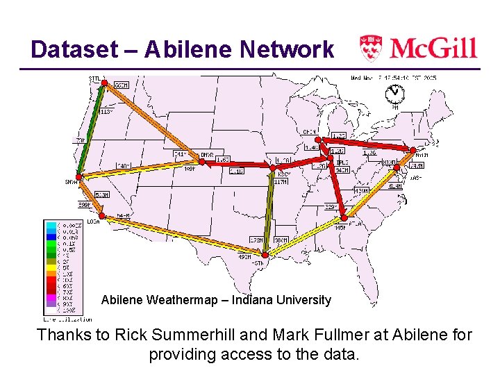
Dataset – Abilene Network Abilene Weathermap – Indiana University Thanks to Rick Summerhill and Mark Fullmer at Abilene for providing access to the data.

Principal Component Analysis (PCA) l Goal: Identify a low-dimensional subspace that captures the key components of the feature set l Idea: If (most of) a measurement does not lie in this subspace, then it is anomalous l PCA l l l conduct a linear transformation to choose a new coordinate system Projection onto first principal component has greater variance than any other projection (maximum energy). Subsequent principal components capture greatest remaining energy

PCA (2) l Reduce dimensionality by eliminating principal components that do not contribute significantly to variance in the dataset (small singular value) l Not optimized for class separability (linear discriminant analysis) l Minimizes reconstruction error under L 2 norm.

“Eigenflow” Analysis l Lakhina et al. (2004, 2004 b). l PCA analysis of Origin-Destination (OD) Flows l Eigenflow: set of flows mapped onto a single principle component l Intrinsic Dimensionality: Empirical studies for Sprint and Abilene networks indicated that 510 principal components sufficed to capture most of the energy.

PCA-based Anomaly Detection l Perform PCA on block of OD flow measurements l Project each measurement onto primary principal components l Test whether the residual energy exceeds a threshold. l Squared prediction error (SPE - Q-statistic) used to test for unusual flow-types. l Prone to Type-I errors (false positives) when applied to transient operations. l In these cases, the assumption that the source data is normally distributed is violated.

Online Method l Don’t need to relearn from scratch when new data arrive l Computational cost per time step should be bounded by constant independent of time l Block-based PCA unattractive l Alternative method: Kernel Recursive Least Squares (KRLS)

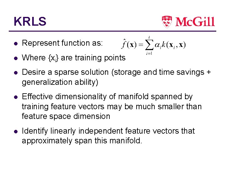
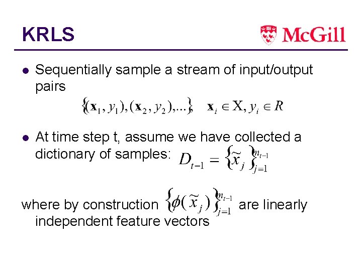
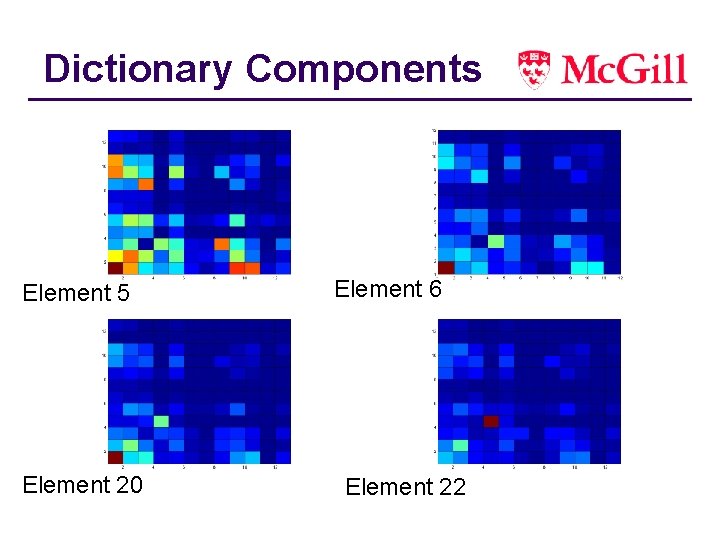
KRLS l Represent function as: l Where {xi} are training points l Desire a sparse solution (storage and time savings + generalization ability) l Effective dimensionality of manifold spanned by training feature vectors may be much smaller than feature space dimension l Identify linearly independent feature vectors that approximately span this manifold.

KRLS l Sequentially sample a stream of input/output pairs l At time step t, assume we have collected a dictionary of samples: where by construction independent feature vectors are linearly

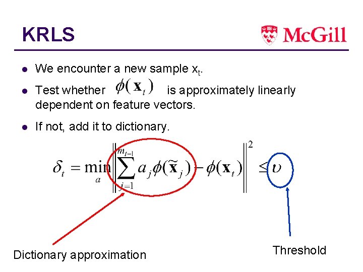
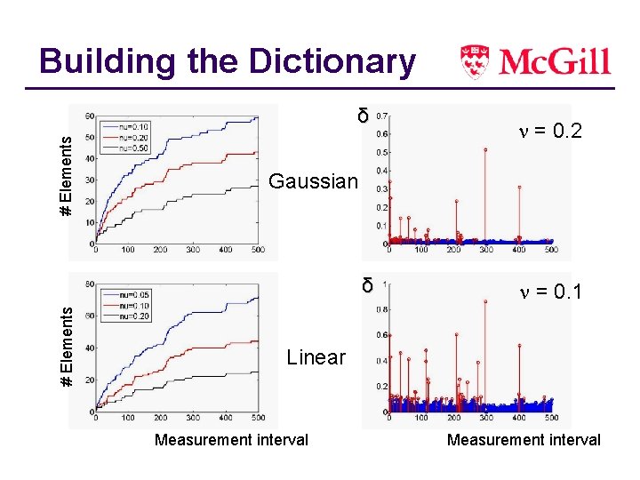
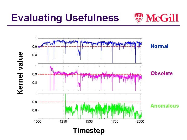
KRLS l We encounter a new sample xt. l Test whether is approximately linearly dependent on feature vectors. l If not, add it to dictionary. Dictionary approximation Threshold

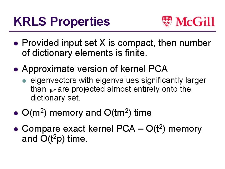
KRLS Properties l Provided input set X is compact, then number of dictionary elements is finite. l Approximate version of kernel PCA l eigenvectors with eigenvalues significantly larger than are projected almost entirely onto the dictionary set. l O(m 2) memory and O(tm 2) time l Compare exact kernel PCA – O(t 2) memory and O(t 2 p) time.

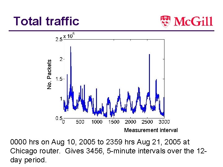
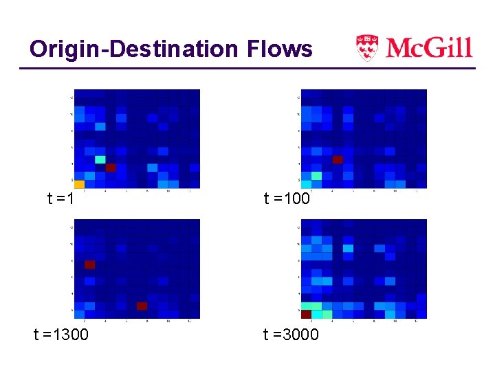
Application in Networks l Data set is the Origin-Destination Flows (11 x 11 matrix = 121 dimensional vector per measurement interval). l Normalized, these comprise the features. l We use the total traffic per measurement interval as the associated value y

No. Packets Total traffic Measurement interval 0000 hrs on Aug 10, 2005 to 2359 hrs Aug 21, 2005 at Chicago router. Gives 3456, 5 -minute intervals over the 12 day period.

Origin-Destination Flows t =100 t =1300 t =3000

Building the Dictionary # Elements δ Gaussian δ # Elements n = 0. 2 n = 0. 1 Linear Measurement interval

Dictionary Components Element 5 Element 20 Element 6 Element 22

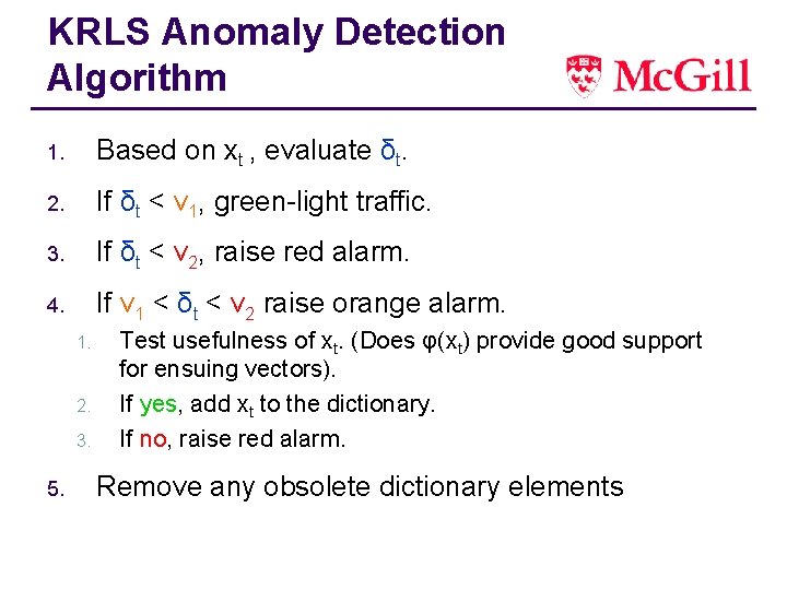
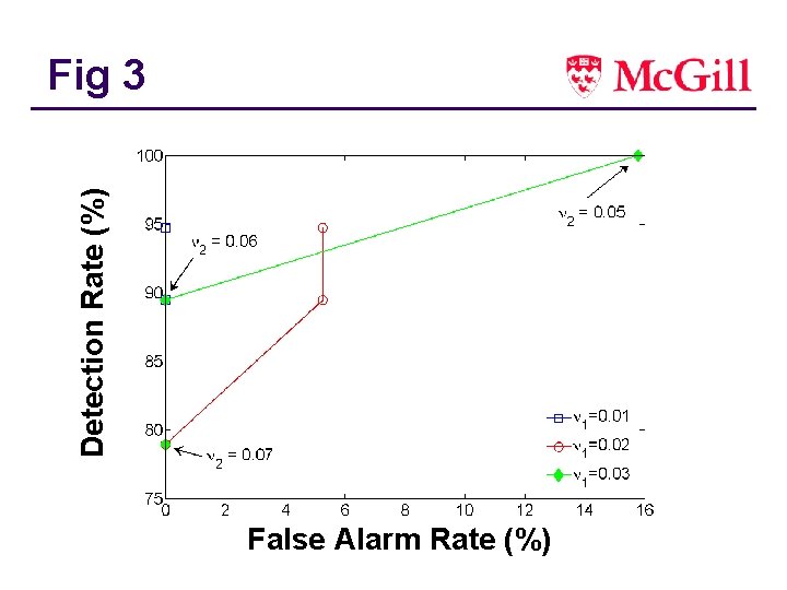
KRLS Anomaly Detection Algorithm 1. Based on xt , evaluate δt. 2. If δt < ν 1, green-light traffic. 3. If δt < ν 2, raise red alarm. 4. If ν 1 < δt < ν 2 raise orange alarm. 1. 2. 3. 5. Test usefulness of xt. (Does φ(xt) provide good support for ensuing vectors). If yes, add xt to the dictionary. If no, raise red alarm. Remove any obsolete dictionary elements

Evaluating Usefulness Kernel value Normal Obsolete Anomalous Timestep

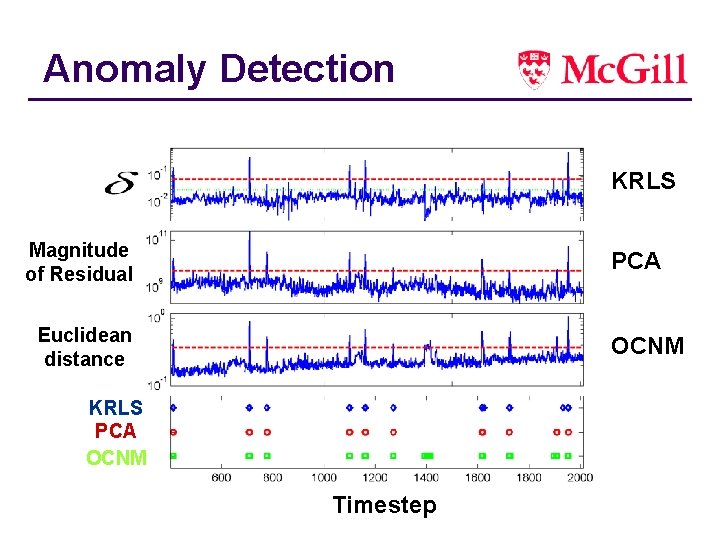
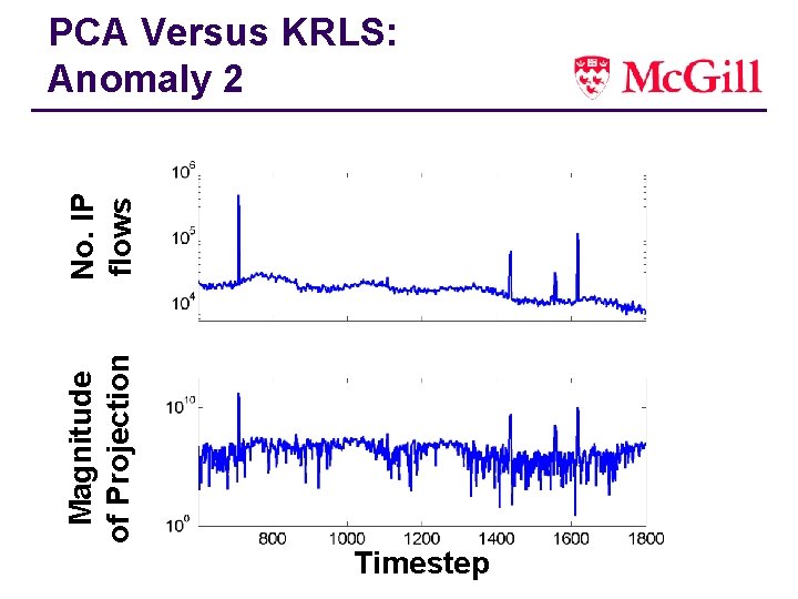
Anomaly Detection KRLS Magnitude of Residual PCA Euclidean distance OCNM KRLS PCA OCNM Timestep

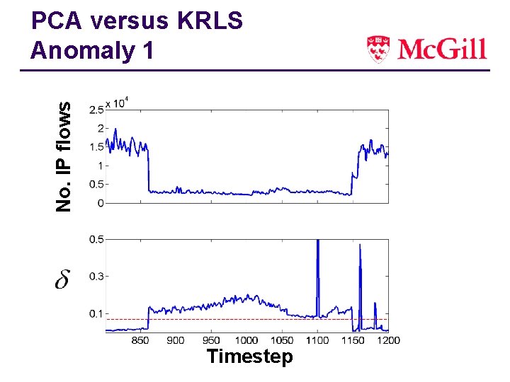
No. IP flows PCA versus KRLS Anomaly 1 Timestep

Magnitude of Projection No. IP flows PCA Versus KRLS: Anomaly 2 Timestep

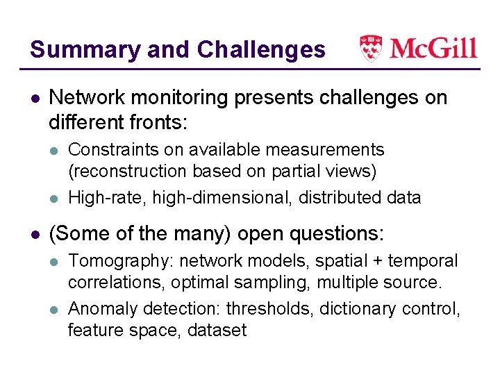
Summary and Challenges l Network monitoring presents challenges on different fronts: l l l Constraints on available measurements (reconstruction based on partial views) High-rate, high-dimensional, distributed data (Some of the many) open questions: l l Tomography: network models, spatial + temporal correlations, optimal sampling, multiple source. Anomaly detection: thresholds, dictionary control, feature space, dataset

Detection Rate (%) Fig 3 False Alarm Rate (%)

Particle filtering Objective: Estimate expectations with respect to a sequence of distributions known up to a normalizing constant, i. e. Monte Carlo: Obtain N weighted samples where such that